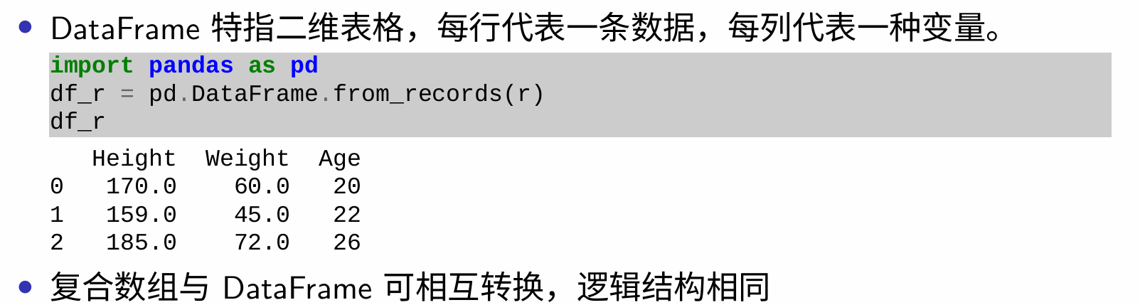
《实验物理的大数据方法》
- git
- git
- commit提交规范
- git cheat sheet
- 其它工具
- python
- 语法
- 科学计算
- 模块
- 工具
- shell
- 大作业
第一步:生成 SSH Key
- 进入 Linux 环境
- 安装 Git 和 SSH:
sudo apt update和sudo apt install git openssh-client - 运行
ssh-keygen,生成一个 SSH Key,一路按照默认回车即可 - 生成的 SSH Key 路径默认是 HOME 路径下的
.ssh/id_rsa.pub和.ssh/id_rsa文件。
第二步:配置 Tsinghua GitLab 的 SSH Key
- 登录 https://git.tsinghua.edu.cn/
- 点击右上角的头像,选择
Preferences - 在左边栏中,点击
SSH Keys - 在终端中运行
cat ~/.ssh/id_rsa.pub,即查看id_rsa.pub文件的内容 - 把输出的内容里,以
ssh-rsa打头的一行,完整复制 - 粘贴到第 3 步的浏览器页面中
- 向 Title 的编辑框内随便写入一个名字
- 点击
Add Key按钮 - 可以看到下面的
Your SSH keys多了一项 - 在终端中运行
ssh -T git@git.tsinghua.edu.cn,即用 SSH Key 来尝试访问 https://git.tsinghua.edu.cn/ - 如果出现了
yes/no的提示,输入yes并回车 - 如果配置成功了,它会显示形如
Welcome to GitLab, @xxx!的提示信息
第三步:克隆仓库
- 访问 https://git.tsinghua.edu.cn/physics-data/2025,在下面寻找有自己名字的仓库,点击进入。点击右侧的蓝色按钮 Clone,下面应该会显示
Clone with SSH和一个文本框,点击右边的按钮进行复制,得到的应该是形如git@git.tsinghua.edu.cn/physics-data/2025/self-intro/self-intro-<USER>.git的内容(其中<USER>代表你的用户名)。如果显示的是 https 开头的内容,要重新回到页面复制正确的 URL。 - 回到终端,输入
git clone 刚才复制的内容(在 WSL 中,可以右键点击窗口标题,选择编辑-粘贴),这时候应该能看到形如git clone git@git.tsinghua.edu.cn/physics-data/2025/self-intro/self-intro-<USER>.git的内容,回车以执行。 - 这时候,你可以输入
ls来列出当前目录的内容,应该可以看到一个新的目录,名字为self-intro-<USER>。你可以输入cd self-intro-<USER>来进入这个目录。 - 再次输入
ls,应该可以看到几个文件:README.mdintroduction.txt和grade.py。这就是这个仓库里的文件了。你马上需要更改的就是introduction.txt的内容。
切换分支
🔍 一、基础切换操作
-
查看分支列表
git branch # 列出本地分支,当前分支前标有 `*` git branch -a # 列出所有分支(本地+远程)作用:确认目标分支名称,避免拼写错误。
-
切换到已存在的分支
git checkout <分支名> # 传统写法 git switch <分支名> # Git 2.23+ 推荐,语义更清晰示例:
git switch dev # 切换到 `dev` 分支注意:若分支不存在,命令会报错。
🛠️ 二、创建并切换到新分支
git checkout -b <新分支名>    # 传统写法
git switch -c <新分支名>      # Git 2.23+ 推荐
示例:
git switch -c feature-login # 创建并切换到 `feature-login` 分支
原理:基于当前分支的最新提交创建新分支,并自动切换。
🔄 三、特殊场景切换技巧
-
切换到上一个分支
git checkout - # 快速返回上一个分支 git switch - # 同上,Git 2.23+ 可用适用场景:临时切换分支后需返回原分支。
-
切换到远程分支
git fetch origin # 先拉取远程分支信息 git switch -c <本地分支名> origin/<远程分支名>示例:
git switch -c hotfix origin/hotfix # 创建本地分支并关联远程 `hotfix`作用:同步远程分支代码到本地新分支。
-
切换到特定提交或标签
git checkout <提交哈希> # 切换到某次提交(进入分离头指针状态) git checkout v1.0 # 切换到标签 `v1.0`注意:此状态下的修改需通过新分支保存,否则可能丢失。
⚠️ 四、切换分支的注意事项
-
未提交修改的处理
- 保存修改:切换前若有未提交的更改,Git 会拒绝切换。需先暂存或提交:
git stash # 暂存修改 git switch dev # 切换分支 git stash pop # 切回后恢复修改 - 强制切换(慎用):
风险:未保存的更改会永久丢失。git checkout -f dev # 丢弃未提交修改,强制切换
- 保存修改:切换前若有未提交的更改,Git 会拒绝切换。需先暂存或提交:
-
冲突预防
若当前分支和目标分支对同一文件有冲突修改,需先解决冲突(如通过git merge或git rebase整合),再切换分支。
💎 五、操作流程示例
# 查看分支
git branch -a        # 输出: * main, origin/dev

# 创建并切换到新分支
git switch -c feature-payment

# 开发并提交代码...
git add .
git commit -m "Add payment module"

# 返回 main 分支
git switch main

# 合并新功能
git merge feature-payment

# 清理分支
git branch -d feature-payment
总结
- 基础切换:优先用
git switch(比git checkout更安全清晰)。 - 关联远程:先
git fetch,再通过git switch -c创建关联分支。 - 未提交修改:务必用
git stash暂存或提交更改,避免数据丢失。 - 冲突处理:切换前确保无文件冲突,必要时手动解决。
一些git commit的options
-m <message>
git commit -m "fix: resolve login timeout issue"
-a / --all
- 作用:自动暂存所有已跟踪文件的修改(不包括新文件),直接提交。
- 场景:跳过
git add步骤,快速提交已知文件的改动。 - 注意:新文件仍需手动
git add。 - 示例:
git commit -am "chore: update config files"
--amend
- 作用:修改最近一次提交(补充漏掉的文件或修正提交信息)。
- 场景:
- 提交后发现有文件遗漏:
git add missing.txt && git commit --amend --no-edit - 提交信息写错:
git commit --amend -m "new message"
- 提交后发现有文件遗漏:
- 风险:若已推送到远程,需
git push -f(可能破坏协作分支的历史)。
-p / --patch
- 作用:交互式选择部分代码块暂存,实现原子提交。
- 场景:单文件含多个逻辑修改时,拆分提交保持清晰。
- 操作:
git add -p  # 按提示选择代码块 (y/n/q)
git commit -m "feat: add user validation"
在团队协作中,规范的 Git Commit 信息是提升沟通效率、代码可维护性和自动化流程的关键。以下基于行业广泛采用的 Conventional Commits 规范(如 Angular 风格)[citation:1][citation:4][citation:5],结合实践建议,为你提供清晰的填写指南:
🧱 一、Commit 信息的核心结构(必含类型)
规范的 Commit 信息通常分为三部分,通过空行分隔:
<类型>(<作用域>): <主题>  // Header(必需)
<空行>
<详细描述>              // Body(可选)
<空行>
<页脚信息>              // Footer(可选)
1. Header(头部):简洁说明修改性质
类型(Type):必填,明确修改的类别,常用类型包括[citation:1][citation:4][citation:8]:
| 类型 | 适用场景 | 是否进 Changelog | |------------|------------------------------------------|---------------------| |feat| 新增功能(feature) | ✅ | |fix| 修复 Bug | ✅ | |docs| 文档更新(README、注释等) | ⚠️ 可选 | |style| 代码格式调整(空格、分号等,不影响逻辑) | ❌ | |refactor| 代码重构(非功能新增或 Bug 修复) | ❌ | |perf| 性能优化 | ✅ | |test| 测试用例新增或修改 | ❌ | |chore| 构建/工具/依赖变更(CI、包管理等) | ❌ | |revert| 回滚某次提交 | ✅ |作用域(Scope):可选,说明影响范围(如模块、文件、功能)- 例:
fix(auth):、feat(router):,无明确范围可用*(如chore(*):)[citation:4][citation:5]。
- 例:
主题(Subject):必填,动词开头的简短描述(≤50字符)- 要求:使用现在时祈使语气(如 "add" 而非 "added")、首字母小写、无句号[citation:1][citation:3]。
2. Body(正文):详细解释修改内容(可选)
- 说明 修改动机、技术细节或前后对比;
- 每行 ≤72 字符,分段清晰[citation:1][citation:4];
- 示例:
重构用户验证逻辑,减少冗余代码:
- 移除重复的权限检查函数;
- 合并身份验证中间件。
3. Footer(页脚):关联问题或破坏性变更(可选)
- 关闭 Issue:
Closes #123[citation:1][citation:5]; - 破坏性变更(Breaking Change):
- 以
BREAKING CHANGE:开头,说明兼容性变化及迁移方案[citation:4][citation:7]; - 或通过在类型后加
!标识(如feat!:)[citation:7]。
- 以
⚙️ 二、团队协作最佳实践
- 原子性提交
一次提交只解决一个问题,避免混合功能、修复或重构,便于回滚和审查[citation:5][citation:10]。 - 关联任务追踪
在主题或页脚中引用任务 ID(如JIRA-123),自动化同步进度[citation:3][citation:6]。 - 分支与提交协同
- 功能开发使用
feat/xxx分支,修复使用fix/xxx分支; - 合并前通过 Pull Request(PR) 进行代码审查[citation:9][citation:10]。
- 功能开发使用
- 自动化工具支持
- 用
commitlint校验信息格式; - 用
standard-version根据类型自动生成 Changelog[citation:4][citation:5]。
- 用
📝 三、示例模板
feat(user): 新增头像上传功能
- 支持本地文件上传及URL导入;
- 添加头像裁剪组件。
BREAKING CHANGE: 移除旧版头像API,改用 `/v2/profile/avatar`。
Closes #45
fix(login): 解决Safari浏览器登录重定向循环
修复因会话Cookie处理不当导致的无限重定向问题,参考MDN安全配置建议。
Fixes #89
💎 四、总结:提升协作效率的关键点
- 类型标准化:用
feat/fix等明确意图,避免模糊词汇(如 "update")[citation:2][citation:5]; - 作用域清晰化:限定影响范围,降低理解成本;
- 主题简洁有力:≤50字符的动词短语概括核心改动;
- 自动化兼容:通过规范格式实现 Changelog 自动生成、Issue 自动关闭[citation:1][citation:4]。
规范 Commit 信息不仅是格式要求,更是团队协作的契约。通过统一语言和结构,开发者能快速定位变更背景、减少沟通摩擦,并为自动化流程铺平道路[citation:6][citation:10]。
tig - text-mode interface for Git
- Git 的增强型前端交互式界面
itg进入交互式界面
键盘输入h进入帮助界面
SYNOPSIS
- tig [options] [revisions] [--] [paths]
- tig log [options] [revisions] [--] [paths]
- tig show [options] [revisions] [--] [paths]
- tig reflog [options] [revisions]
- tig blame [options] [rev] [--] path
- tig grep [options] [pattern]
- tig refs [options]
- tig stash [options]
- tig status
- tig < [Git command output]
==用于比较两个对象的值是否相等,is用于比较两个对象的id值是否相等,即是否位于同一地址。bool(-6) # => True-5 != False # => True-5 or 0 # => -52 < 3 < 2 # => False
# Strings can be added too
"Hello " + "world!"  # => "Hello world!"
# String literals (but not variables) can be concatenated without using '+'
"Hello " "world!"    # => "Hello world!"
# You can find the length of a string
len("This is a string")  # => 16
# Don't use the equality "==" symbol to compare objects to None
# Use "is" instead. This checks for equality of object identity.
"etc" is None  # => False
None is None   # => True
print的可选参数
# By default the print function also prints out a newline at the end.
# Use the optional argument end to change the end string.
print("Hello, World", end="!")  # => Hello, World!
if,else可以作为表达式
# if can be used as an expression
# Equivalent of C's '?:' ternary operator
"yay!" if 0 > 1 else "nay!"  # => "nay!"
列表
- 列表中的元素类型可以是不同的
- 列表的元素用
,分隔,最后,之后再添加空格,优化代码风格
列表的append和pop方法
# Add stuff to the end of a list with append
li.append(1)    # li is now [1]
li.append(2)    # li is now [1, 2]
li.append(4)    # li is now [1, 2, 4]
li.append(3)    # li is now [1, 2, 4, 3]
# Remove from the end with pop
li.pop()        # => 3 and li is now [1, 2, 4]
# Let's put it back
li.append(3)    # li is now [1, 2, 4, 3] again.
列表的切片
li[::2]   # Return list selecting elements with a step size of 2 => [1, 4]
li[::-1]  # Return list in reverse order => [3, 4, 2, 1]
# li[start:end:step]
- list两个冒号的用法(numpy数组类似)
- 第一个index指定开始,第二个index指定结束,第三个指定间隔
ls = list(range(100))

ls[0:100:10]
# [out]:[0, 10, 20, 30, 40, 50, 60, 70, 80, 90]
删除列表中的元素
# 按位置删除
# Remove arbitrary elements from a list with "del"
del li[2]  # li is now [1, 2, 3]

# 按值删除
# Remove first occurrence of a value
li.remove(2)  # li is now [1, 3]
li.remove(2)  # Raises a ValueError as 2 is not in the list
清空列表
li.clear() # Remove all elements from the list
删除列表对象
del li # Delete the list object
在列表中插入元素
# 第一个参数为位置,第二个参数为值
# Insert an element at a specific index
li.insert(1, 2)  # li is now [1, 2, 3] again
列表加法
# You can add lists
# Note: values for li and for other_li are not modified.
li + other_li  # => [1, 2, 3, 4, 5, 6]

# Concatenate lists with "extend()"
li.extend(other_li)  # Now li is [1, 2, 3, 4, 5, 6]
列表的其他操作
# Check for existence in a list with "in"
1 in li  # => True

# Examine the length with "len()"
len(li)  # => 6
元组
- 类似列表但是不能更改值:没有
append()方法 - 但是有定义加法这很奇怪:产生了一个新的元组,但是原来的元组并没有被改变
tup = (1, 2, 3)
tup[0]      # => 1
tup[0] = 3  # Raises a TypeError
list = [1, 2, 3]

tu = tuple(list); print(tu) # => (1, 2, 3)
tu += (4,); print(tu) # => (1, 2, 3, 4)
- 元组的小陷阱
# Note that a tuple of length one has to have a comma after the last element but
# tuples of other lengths, even zero, do not.
type((1))   # => <class 'int'>
type((1,))  # => <class 'tuple'>
type(())    # => <class 'tuple'>
使用与列表的操作在元组上一般都能使用
元组的解包
# You can unpack tuples (or lists) into variables
a, b, c = (1, 2, 3)  # a is now 1, b is now 2 and c is now 3
# You can also do extended unpacking
a, *b, c = (1, 2, 3, 4)  # a is now 1, b is now [2, 3] and c is now 4
# Tuples are created by default if you leave out the parentheses
d, e, f = 4, 5, 6  # tuple 4, 5, 6 is unpacked into variables d, e and f
# respectively such that d = 4, e = 5 and f = 6
# Now look how easy it is to swap two values
e, d = d, e  # d is now 5 and e is now 4
字典
左key右value
- 为了保证字典的正确性和稳定性,键需要是不可变类型,常见的不可变类型包括整数、浮点数、字符串、元组,因为这些类型在创建后其值不能被改变,这样可以确保字典的键在使用过程中保持唯一性和稳定性。
value可以是任何类型
字典的查看:[]
# Look up values with []
filled_dict["one"]  # => 1
字典的快捷构造方法
- 可以使用任何输出序对的迭代器构造字典
dict(enumerate("abcd"))
直接对字典进行迭代,输出的是Key
使用“keys()”、“values()”方法获取所有键作为可迭代对象。我们需要将其调用用 list() 包裹起来,将其转换为列表。
list(filled_dict.keys())
list(filled_dict.values())
items()方法,将键值对一起迭代
for key, value in filled_dict.items():
    print(key, value)
使用get()方法避免KeyError,还可以设置defult值
# Looking up a non-existing key is a KeyError
filled_dict["four"]  # KeyError

# Use "get()" method to avoid the KeyError
filled_dict.get("one")      # => 1
filled_dict.get("four")     # => None
# The get method supports a default argument when the value is missing
filled_dict.get("one", 4)   # => 1
filled_dict.get("four", 4)  # => 4
setdefault()方法
- 先检查字典中是否存在“key”这个键。如果不存在,就会将“key”和对应的“value”插入到字典中;如果“key”已经存在,那么就不会插入,字典保持不变。
filled_dict.setdefault("five", 5)  # filled_dict["five"] is set to 5
filled_dict.setdefault("five", 6)  # filled_dict["five"] is still 5
字典的删除:del,dic = {},dic.pop(keys),dic.popitem()
字典的更新
# Adding to a dictionary
filled_dict.update({"four":4})  # => {"one": 1, "two": 2, "three": 3, "four": 4}
filled_dict["four"] = 4         # another way to add to dict

# Remove keys from a dictionary with del
del filled_dict["one"]  # Removes the key "one" from filled dict
字典的作用:条件语句字典化
aff = '工物'
if aff == '工物':
    print(20)
elif aff == '物理':
    print(40)
elif aff == "上海交大":
    print(2)
else:
    print(1)

# 用字典查询更加方便
print(sc[aff])
set集合
集合的声明
empty_set = set()
# Initialize a set with a bunch of values.
some_set = {1, 1, 2, 2, 3, 4}  # some_set is now {1, 2, 3, 4}
集合中的元素可以是不同类型的,但是必须是不可变类型
invalid_set = {[1], 1}  # => Raises a TypeError: unhashable type: 'list'
valid_set = {(1,), 1}
集合中添加元素
# Add one more item to the set
filled_set = some_set
filled_set.add(5)  # filled_set is now {1, 2, 3, 4, 5}
# Sets do not have duplicate elements
filled_set.add(5)  # it remains as before {1, 2, 3, 4, 5}
集合之间的交并补运算
- 集合取交集
# Do set intersection with &
other_set = {3, 4, 5, 6}
filled_set & other_set  # => {3, 4, 5}
- 集合取并集
# Do set union with |
filled_set | other_set  # => {1, 2, 3, 4, 5, 6}
- 集合取补集
# Do set difference with -
{1, 2, 3, 4} - {2, 3, 5}  # => {1, 4}

# Do set symmetric difference with ^
{1, 2, 3, 4} ^ {2, 3, 5}  # => {1, 4, 5}
- 集合的包含关系
# Check if set on the left is a superset of set on the right
{1, 2} >= {1, 2, 3}  # => False

# Check if set on the left is a subset of set on the right
{1, 2} <= {1, 2, 3}  # => True
- 集合是可变的
A = {1, 2, 3}
A.add(4)  # A is now {1, 2, 3, 4}
A.discard(2)  # A is now {1, 3, 4}
A.clear()  # A is now set()
A.pop()
字符串
str.strip()方法:移除字符串首尾的指定字符(默认空白符)
defaultdict–带有默认值的字典
from collections import defaultdict
dsc = defaultdict(int)
- The default factory is called without arguments to produce a new value when a key is not present, in getitem only. A defaultdict compares equal to a dict with the same items. All remaining arguments are treated the same as if they were passed to the dict constructor, including keyword arguments.
Counter–计数器
- Dict subclass for counting hashable items. Sometimes called a bag or multiset. Elements are stored as dictionary keys and their counts are stored as dictionary values.
eps = ["物理","物理","工物","工物","物理"]
from collections import Counter
 cnumbers = Counter(deps)
 print(cnumbers)
- Counter({'物理':3,'工物':2})
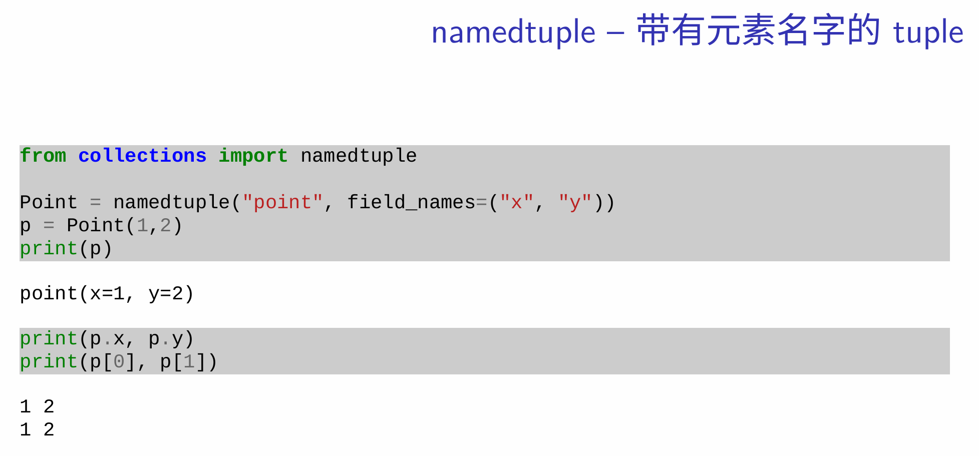
带名字的tuple
一些其他很python的用法
list comprehensions列表推导式
[add_10(i) for i in [1, 2, 3]]         # => [11, 12, 13]
[x for x in [3, 4, 5, 6, 7] if x > 5]  # => [6, 7]
- 集合和字典都可以如此使用
{x for x in "abcddeef" if x not in "abc"}  # => {'d', 'e', 'f'}
{x: x**2 for x in range(5)}  # => {0: 0, 1: 1, 2: 4, 3: 9, 4: 16}
if else语句
if some_var > 10:
    print("some_var is totally bigger than 10.")
elif some_var < 10:    # This elif clause is optional.
    print("some_var is smaller than 10.")
else:                  # This is optional too.
    print("some_var is indeed 10.")
Match/Case语句
command = "run"
match command:
case "run":
print("The robot started to run 🏃♂️")
case "speak" | "say_hi": # multiple options (OR pattern)
print("The robot said hi 🗣️")
case code if command.isdigit(): # conditional
print(f"The robot execute code: {code}")
case _: # _ is a wildcard that never fails (like default/else)
print("Invalid command ❌")
for循环语句
- 循环语句需要迭代器,迭代器可以是列表,也可以使用range()函数生成顺序数字组成的列表。
for animal in ["dog", "cat", "mouse"]:
    # You can use format() to interpolate formatted strings
    print("{} is a mammal".format(animal))

for i in range(4):
    print(i)
for i in range(4, 8):
    print(i)
for i in range(4, 8):
    print(i)
- 将列表中元素的
index和value一起进行迭代
animals = ["dog", "cat", "mouse"]
for i, value in enumerate(animals):
    print(i, value)
while循环语句
x = 0
while x < 4:
    print(x)
    x += 1  # Shorthand for x = x + 1
可迭代iterable对象
filled_dict = {"one": 1, "two": 2, "three": 3}
our_iterable = filled_dict.keys()
注意可迭代对象不能通过Index取值
our_iterable[1] # Raises a TypeError
可迭代对象可以用来构造迭代器iter()函数
our_iterator = iter(our_iterable)
迭代器的next()函数可以获取下一个元素
print(next(our_iterator)) # "one"
StopIteration异常:当迭代器已将迭代完后再对其进行迭代
注意区分可迭代对象和由iter()生成的迭代器
# You can grab all the elements of an iterable or iterator by call of list().
list(our_iterable)  # => Returns ["one", "two", "three"]
list(our_iterator)  # => Returns [] because state is saved
函数定义
# Use "def" to create new functions
def add(x, y):
    print("x is {} and y is {}".format(x, y))
    return x + y  # Return values with a return statement
- 以上这个函数对字符串也适用,但是我们不想要字符串,只需要整数相加?
def add(x: int, y: int) -> int:
    print("x is {} and y is {}".format(x, y))
    return x + y  # Return values with a return statement
- 然而只是方便阅读……自由派python鼓励大家把类型标注上,但是类型不匹配的时候也不会报错
python函数的参数是否会在内部改变?
- 对于list,字典等可变对象,变量像C语言中的指针一样会改变,对于不可变对象则类似于复制传值,外部的变量不会改变
map()函数
- map(func, *iterables) --> map object
- Make an iterator that computes the function using arguments from each of the iterables. Stops when the shortest iterable is exhausted.
- 从一个迭代器,经过一个函数映射到另一个迭代器
def squared(x):
    return x*x

list(map(squared, [1,2,3,4,5,6]))
lazy evaluate策略:节省内存
In [49]: def sqr(x):
    ...:     return x*x
    ...: map(sqr,range(4))
Out[49]: <map at 0x765d78b17dc0>
- range()返回的是一个迭代器类型,也采用laze evaluate策略,map()之后的也是一个lazy策略的迭代器
这很python!!!!
可以接受任意(可变)数量位置的函数
# You can define functions that take a variable number of
# positional arguments
def varargs(*args):
    return args
可以接受任意(可变)数量关键字参数的函数
# You can define functions that take a variable number of
# keyword arguments, as well
def keyword_args(**kwargs):
    return kwargs
上述两种定义方式的组合
# You can do both at once, if you like
def all_the_args(*args, **kwargs):
    print(args)
    print(kwargs)

all_the_args(1, 2, a=3, b=4) prints:
    (1, 2)
    {"a": 3, "b": 4}
函数调用时解包参数
# Use * to expand args (tuples) and use ** to expand kwargs (dictionaries).
args = (1, 2, 3, 4)
kwargs = {"a": 3, "b": 4}
all_the_args(*args)            # equivalent: all_the_args(1, 2, 3, 4)
all_the_args(**kwargs)         # equivalent: all_the_args(a=3, b=4)
all_the_args(*args, **kwargs)  # equivalent: all_the_args(1, 2, 3, 4, a=3, b=4)
通过元组解包返回多个值
# Returning multiple values (with tuple assignments)
def swap(x, y):
    return y, x  # Return multiple values as a tuple without the parenthesis.
                 # (Note: parenthesis have been excluded but can be included)
- 返回多个值:在Python中,可以通过返回一个元组来返回多个值。
- 元组解包:可以使用元组解包将返回的多个值分别赋给不同的变量。
- 语法灵活性:返回多个值时,可以省略圆括号,但返回值仍然是一个元组。
名字空间
# global scope
x = 5

def set_x(num):
    # local scope begins here
    # local var x not the same as global var x
    x = num    # => 43
    print(x)   # => 43

def set_global_x(num):
    # global indicates that particular var lives in the global scope
    global x
    print(x)   # => 5
    x = num    # global var x is now set to 6
    print(x)   # => 6
- 强行使用全局变量:在函数体内通过
global varable声明全局变量。
非常不推荐
无名函数lambda:常用于与map()配合使用
map(square, range(6))
first class function头等函数
- 头等函数:可以作为参数传递,也可以作为返回值返回
def create_adder(x):
    def adder(y):
        return x + y
    return adder

add_10 = create_adder(10)
add_10(3)   # => 13
Closures in nested functions嵌套函数中的闭包
嵌套函数
def outer(x):
    def inner(y):
        return x + y  # inner访问outer的变量x
    return inner
closure = outer(10)
print(closure(5))  # 输出15[1,2](@ref)
- 内部函数可访问外部函数的变量(词法作用域),但外部函数不能直接访问内部函数的变量
闭包
- 内部函数携带外部函数的环境(变量),即使外部函数已执行完毕(如计数器、惰性求值)
def create_avg():
    total = 0
    count = 0
    def avg(n):
        nonlocal total, count
        total += n
        count += 1
        return total/count
    return avg
avg = create_avg()
avg(3)  # => 3.0
avg(5)  # (3+5)/2 => 4.0
avg(7)  # (8+7)/3 => 5.0
# We use the "class" statement to create a class
class Human:

    species = "H. sapiens"
- 类的属性
attribute,被所有实例共享
    def __init__(self, name):
        # Assign the argument to the instance's name attribute
        self.name = name

        # Initialize property
        self._age = 0
- 构造函数里面的变量才是每个对象独有的属性
- 前面带下划线的属性提示这是一个私有属性,只在类的内部方法使用(但是python……你懂的,只是建议)
    def say(self, msg):
        print("{name}: {message}".format(name=self.name, message=msg))
- 实例方法,第一个参数是实例本身,可以访问实例的属性和方法
    # A class method is shared among all instances
    # They are called with the calling class as the first argument
    @classmethod
    def get_species(cls):
        return cls.species
- 类方法,第一个参数是类本身,可以访问类的属性和方法
    # A static method is called without a class or instance reference
    @staticmethod
    def grunt():
        return "*grunt*"
- 静态方法,不依赖于实例或类,可以像普通函数一样被调用,但它们属于类的命名空间,而不是类的实例。
- 静态方法与类相关联,但是关联性最弱 -可以直接通过类名来调用它,而不需要创建类的实例。
对于实例内部私有属性的方法
    # A property is just like a getter.
    # It turns the method age() into a read-only attribute of the same name.
    # There's no need to write trivial getters and setters in Python, though.
    @property
    def age(self):
        return self._age
- 用
@property装饰器装饰的方法,可以像属性一样访问,但是不能像方法一样调用。 - 但是可以通过属性名来调用它,这就是为什么我们可以用
obj.age来访问对象的年龄,而不需要obj.get_age()。
    # This allows the property to be set
    @age.setter
    def age(self, age):
        self._age = age

    # This allows the property to be deleted
    @age.deleter
    def age(self):
        del self._age
使用名字空间判断语句在程序启动时自动创建实例
# When a Python interpreter reads a source file it executes all its code.
# This __name__ check makes sure this code block is only executed when this
# module is the main program.
if __name__ == "__main__":
    # Instantiate a class
    i = Human(name="Ian")
    i.say("hi")                     # "Ian: hi"
    j = Human("Joel")
    j.say("hello")                  # "Joel: hello"
    # i and j are instances of type Human; i.e., they are Human objects.

    # Call our class method
    i.say(i.get_species())          # "Ian: H. sapiens"
    # Change the shared attribute
    Human.species = "H. neanderthalensis"
    i.say(i.get_species())          # => "Ian: H. neanderthalensis"
    j.say(j.get_species())          # => "Joel: H. neanderthalensis"

    # Call the static method
    print(Human.grunt())            # => "*grunt*"

    # Static methods can be called by instances too
    print(i.grunt())                # => "*grunt*"

    # Update the property for this instance
    i.age = 42
    # Get the property
    i.say(i.age)                    # => "Ian: 42"
    j.say(j.age)                    # => "Joel: 0"
    # Delete the property
    del i.age
实现迭代器
- 实现“迭代器协议”,在类中定义__iter__() 函数和__next__()函数
class Fibonacci:
    def __init__(self, n):
        self.n = n
        self.a, self.b = 0, 1

    def __iter__(self):
        return self

    def __next__(self):
        fib = self.a
        if fib > self.n:
            raise StopIteration
        self.a, self.b = self.b, self.a + self.b
        return fib
- 实现“迭代器协议”的类,必须实现两个方法:
__iter__()和__next__()。 __iter__()方法返回一个迭代器对象,该对象实现了__next__()方法。__next__()方法返回迭代器的下一个值,或者在迭代结束时引发StopIteration异常。- 迭代器对象可以被用于
for循环,或者用next()函数来获取下一个值。
fib = Fibonacci(100)
for num in fib:
    print(num)
类的继承与封装
等有需要再来学吧
类与对象的一些用法
使用类封装全局变量
dict_keys视图对象
在Python中,dic.keys()返回的类型是视图对象(view object),具体类型名为dict_keys。以下是详细解释:
🔍 1. dict_keys类型的基本特性
-
动态视图:
dic.keys()返回的是一个动态视图对象(dict_keys),而非静态列表或元组。它会实时反映字典键的变化:当字典内容被修改(如增删键)时,视图对象会自动更新[citation:2][citation:6][citation:7][citation:10]。dic = {'a': 1, 'b': 2} keys_view = dic.keys() print(type(keys_view)) # <class 'dict_keys'> dic['c'] = 3 # 修改字典 print(keys_view) # dict_keys(['a', 'b', 'c']) → 自动更新 -
内存高效:
由于不生成数据副本,dict_keys对大型字典更高效。例如,一个包含100万键的字典,keys()直接返回视图(几乎不占额外内存),而转换为列表需复制所有键[citation:7][citation:9]。
🔧 2. 核心功能与操作
-
可迭代性:
dict_keys支持迭代操作,可直接用于循环:for key in dic.keys(): print(key, dic[key])等价于
for key in dic:,但显式使用keys()更清晰[citation:2][citation:4]。 -
集合式操作:
dict_keys支持集合运算(交集、并集、差集),行为类似集合(set)[citation:10]:dic1 = {'a': 1, 'b': 2} dic2 = {'b': 2, 'c': 3} print(dic1.keys() & dic2.keys()) # {'b'} → 交集 print(dic1.keys() - dic2.keys()) # {'a'} → 差集 -
成员检测:
可直接用in判断键是否存在,效率与字典本身相同(O(1)时间复杂度):if 'a' in dic.keys(): # 等价于 if 'a' in dic: print("Key exists")
⚠️ 3. 与Python 2的区别
- Python 2:
keys()返回静态列表(list),修改字典不会更新该列表[citation:7][citation:9]。 - Python 3:
改为返回动态视图dict_keys,更节省内存且支持实时更新[citation:7][citation:9][citation:10]。
🛠️ 4. 实际应用场景
- 遍历键并操作字典:
动态视图确保迭代时始终访问最新键,但需注意:遍历中修改字典大小(增删键)会引发RuntimeError[citation:10]。 - 获取键的快照:
需静态副本时,可显式转换为列表:keys_list = list(dic.keys()) # 生成独立列表 - 键的集合运算:
利用&、|、-快速比较多个字典的键关系[citation:10]。
⚠️ 5. 注意事项
- 不可直接索引:
dict_keys不支持索引(如keys_view[0]会报错),需先转为列表[citation:9]。 - 非哈希性:
视图对象本身不可哈希(不能作为字典键或集合元素)[citation:10]。
💎 总结
| 特性 | 说明 |
|---|---|
| 类型 | dict_keys(动态视图对象) |
| 内存效率 | 高效,不复制数据 |
| 动态更新 | 随字典修改自动更新 |
| 主要操作 | 迭代、集合运算、成员检测 |
| 转换静态列表 | list(dic.keys()) |
- 若需操作独立副本(如避免修改干扰),务必转换为列表;若需实时同步字典状态,直接使用视图更高效
生成器
# Generators help you make lazy code.
def double_numbers(iterable):
    for i in iterable:
        yield i + i

for i in double_numbers(range(1, 900000000)):  # `range` is a generator.
    print(i)
    if i >= 30:
        break
yield是生成器的关键特性,它允许函数在每次调用时返回一个值,而不是一次性返回所有值。每次调用生成器时,它会从上次 yield 的地方继续执行,而不是从头开始。range()本身也是一个生成器
生成器表达式
values = (-x for x in [1,2,3,4,5])
for x in values:
    print(x)  # prints -1 -2 -3 -4 -5 to console/terminal
装饰器
装饰器基于闭包实现,用于增强函数行为而不修改原函数代码。
- 基本结构
- 接收函数,返回增强后的新函数(常结合
functools.wraps保留元数据)
from functools import wraps def log_decorator(func): @wraps(func) def wrapper(*args, **kwargs): print(f"调用 {func.__name__}") return func(*args, **kwargs) return wrapper - 接收函数,返回增强后的新函数(常结合
- 类型扩展
- 带参装饰器:嵌套三层(参数→装饰器→包装函数)
def repeat(n): def decorator(func): def wrapper(): for _ in range(n): func() return wrapper return decorator - 类装饰器:通过
__call__方法实现
- 带参装饰器:嵌套三层(参数→装饰器→包装函数)
- 典型场景
- 日志/性能监控:记录函数执行时间和参数
- 权限校验:在敏感操作前检查用户权限
- 结果缓存:存储函数返回值避免重复计算
try-except语句
# Handle exceptions with a try/except block
try:
    # Use "raise" to raise an error
    raise IndexError("This is an index error")
except IndexError as e:
    pass                 # Refrain from this, provide a recovery (next example).
except (TypeError, NameError):
    pass                 # Multiple exceptions can be processed jointly.
else:                    # Optional clause to the try/except block. Must follow
                         # all except blocks.
    print("All good!")   # Runs only if the code in try raises no exceptions
finally:                 # Execute under all circumstances
    print("We can clean up resources here")
文件操作
- python和shell文件操作的基本思想:文件是迭代器,逐行。每行是字符串。
with语句用于文件读写
with语句可以自动关闭文件,避免忘记关闭文件造成资源泄露。
# Instead of try/finally to cleanup resources you can use a with statement
with open("myfile.txt") as f:
    for line in f:
        print(line)
文件写入
- 两种格式:字符串格式和json格式
- 字符串格式:简单直接,但读取时需要手动解析字符串。
- json格式:易于读取和解析,适合与其他程序或语言交互。
# Writing to a file
contents = {"aa": 12, "bb": 21}
with open("myfile1.txt", "w") as file:
    file.write(str(contents))        # writes a string to a file

import json
with open("myfile2.txt", "w") as file:
    file.write(json.dumps(contents))  # writes an object to a file
文件读取
# Reading from a file
with open("myfile1.txt") as file:
    contents = file.read()           # reads a string from a file
print(contents)
# print: {"aa": 12, "bb": 21}

with open("myfile2.txt", "r") as file:
    contents = json.load(file)       # reads a json object from a file
print(contents)
# print: {"aa": 12, "bb": 21}
pathlib中的 Path 类读写
from pathlib import Path

path = Path('data.txt')
contents = path.read_text() # 类型为 <class 'str'>
lines = contents.splitlines() # 类型为 <class 'list'>

path.write_text("I love programing.") # 只能写入str
path.write_text("I hate programing.") # 此时文件内的内容只有"I hate programing."
文件写入的注意事项
- 若文件已存在,清空其所有内容,再写入新数据;若文件不存在,创建新文件后写入。
- 每次
path.write_text()或者open("myfile2.txt", "w") as file都会覆盖文件之前的内容 path.write_text()只支持一次写入,不支持多次写入open("myfile2.txt", "a"):使用追加模式可以避免已存在文件被覆盖
sys.argv
$ ./sys_demo.py 1 2 4 "Hellow, this is command."

<class 'list'>
['./sys_demo.py', '1', '2', '4', 'Hellow, this is command.']
函数的文档
def spherical_harmonic_fitter(grid, order):
    "求球谐函数拟合的系数"

    # 具体实现省略
    pass

help(spherical_harmonic_fitter)
- 通过
help(function_name)读取函数文档
Help on function spherical_harmonic_fitter in module __main__:

spherical_harmonic_fitter(grid, order)
    求球谐函数拟合的系数
- 同理在类与对象的定义中也有类似的文档字符串的用法。
- 更多的注释:使用三引号
def function_name(parameter_list):
    """
    中间是一大串文档,可以使用单个"
    """
    # 函数实现代码
    pass
Numpy Array对象
- ndarray是不可变对象
1. ndarray类的基本属性
- shape:元组
- size:数组中元素的总数
- ndim:维度的数量
- nbytes:存储数据的字节数
- dtype:数组中元素的数据类型
2. 数据类型
| dtype | 变体 | 说明 |
|---|---|---|
| int | intn(n = 8, 16, 32, ···) | |
| uint | uintn(n = 8, 16, 32, ···) | 无符号整型 |
| bool | Bool | |
| float | floatn | 浮点类型 |
| complex | complexN | 复数浮点型 |
- 还支持其他非数字类型:字符串、对象等
- 默认的数据类型是float
- ndarray对象创建后的dtype不能更改,除非复制数组进行类型转换:
data = np.array([1, 2, 3],dtype = np.float) # 类型转换 data = np.array(data, dtype = np.int)- 也可以使用
astype方法:
data.astype(np.int) - 也可以使用
- 在进行运算时,数据类型可能会发生转变。
- 将浮点类型与复数浮点类型——>复数类型
实部与虚部
- 不管的type的类型是什么,ndarray实例都具有real和imag属性
创建数组
| 函数名 | 数组类型 |
|---|---|
| np.arry | 使用类数组对象创建 |
| np.zeros | |
| np.ones | |
| np.fill | 创建指定数值填充的数组 |
| np.diag | |
| np.arange | 指定开始值,结束值以及增量值(不包含结束值) |
| np.linspace | 指定开始值,结束值,元素数量(包含结束值) |
| np.logspace | 等比数列,指定开始值和结束值是可选参数base的幂次(默认为10) |
| np.meshgrid | 从一维坐标向量生成坐标矩阵(或高维坐标数组) |
| np.fromfunction | |
| np.fromfile | |
| np.loadtxt | 从文本文件读取数据以创建数组 |
| np.genfromtxt | 相比于loadtxt,还支持处理缺失值 |
| np.random.rand | 0,1之间分布的随机数 |
meshgrid
将一维坐标向量转换为多维网格坐标矩阵,便于在多维空间中计算和可视化。
网格生成机制
给定一维向量 x(长度 m)和 y(长度 n),meshgrid 输出两个矩阵:
X:每行复制x,共 n 行(y的长度),形状为(n, m)。Y:每列复制y,共 m 列(x的长度),形状为(n, m)。
示例:
import numpy as np
x = [1, 2, 3]; y = [4, 5]
X, Y = np.meshgrid(x, y)
输出:
X = [[1, 2, 3],
     [1, 2, 3]]  # 每行重复 x
Y = [[4, 4, 4],
     [5, 5, 5]]  # 每列重复 y
几何意义:网格点坐标为 (X[i,j], Y[i,j]),覆盖所有组合(如 (1,4), (2,4), (3,4), (1,5)...)。
参数解析
1. 索引模式 indexing
'xy'(默认,笛卡尔坐标):输出形状为(n, m),适合绘图(X为横轴,Y为纵轴)。'ij'(矩阵索引):输出形状为(m, n),适合矩阵运算(如线性代数)。
示例:
X_xy, Y_xy = np.meshgrid(x, y)          # 形状 (2,3)
X_ij, Y_ij = np.meshgrid(x, y, indexing='ij')  # 形状 (3,2)
2. 高维扩展
支持三维网格生成:
x = [1, 2]; y = [3, 4]; z = [5, 6]
X, Y, Z = np.meshgrid(x, y, z)  # 输出形状 (2,2,2)
典型应用场景
1. 绘制等高线图(Contour Plot)
import matplotlib.pyplot as plt
x = np.linspace(-3, 3, 100)
y = np.linspace(-3, 3, 100)
X, Y = np.meshgrid(x, y)
Z = np.sin(X**2 + Y**2)  # 计算网格点函数值
plt.contourf(X, Y, Z, cmap='viridis')
plt.colorbar()
plt.show()
关键:X, Y 定义网格坐标,Z 为每个点的计算值。
使用其他数组的属性创建相同属性的数组
np.ones_like、np.zeros_like、np.full_like、np.empty_like
创建矩阵数组
np.identity:生成单位矩阵np.eye:生成对角线为1的矩阵,偏移量为可选参数np.eye(5,k = 1) np.eye(5,k = -1)np.diag:创建对角线为任意一维数组的函数,也可指定偏移量(关键字k)
索引和切片
视图
- 使用切片操作从数组中提取的子数组是同一底层数组数据的视图。也就是说,它们引用的是原始数组在内存中的同一份数据,但是具有不同的stides设置。视图中的元素被赋予新值后,原始数组中的值也会随之更新。
- 当需要的是数组的副本而不是视图时,应该使用ndarray的copy方法显式地复制视图
C = B[1:10 1:10].copy()
花式索引fancy indexing
- 可以使用另外一个Numpy数组、Python列表、整数序列进行索引
A = linespace(0,1,11)
A[np.array([0,2,4])] # 取出index为0,2,4的元素
布尔索引
- 索引操作可以很好地和布尔操作结合起来
A[A > 0.5]
- 花式索引和布尔索引得到的不是视图,而是新的独立数组
- 可以使用花式索引和布尔索引来改变所选元素,对其赋值会改变原数组元素的值
调整形状和大小
| 函数/方法 | 说明 |
|---|---|
| np.reshape和np.ndarray.reshape | |
| np.ndarray.flatten | 创建副本,并折叠为一维数组 |
| np.ravel和np.ndarray.ravel | 创建视图,并折叠为一维数组 |
| np.squeeze | 删除长度为1的维度 |
| np.expand_dims和np.newaxis | 增加长度为1的维度 |
| np.transpose,np.ndarray.transpose和np.ndarray.T | 对数组进行转置,即对相应的轴进行反转 |
| np.hstack | 水平叠加,沿着轴1 |
| np.vstack | 垂直叠加,沿着轴0 |
| np.dstack | 深度叠加,沿着轴2 |
| np.concatenate | 沿着给定轴堆叠 |
| np.resize | 根据给定的大小创建原始数组的新副本 |
| np.append | 在数组中添加新元素(会创建新副本) |
| np.insert | |
| np.delete |
使用索引表达式和 np.newaxis 关键字添加新的空轴
data = np.arange(0,5)
column = data[:, np.newaxis]
np.expand_axis(data, axis=1)

row = data[np.newaxis, :]
np.expand_axis[data, axis=0]
数组的拼接和堆叠
- 堆叠函数
data = np.arange(5)
np.vstack(data, data, data)
np.stack()堆叠
一、函数原型与参数
numpy.stack(arrays, axis=0)
arrays:需堆叠的数组序列(列表或元组),所有数组形状必须相同。axis:指定新轴插入位置(默认axis=0)。取值范围为[-ndim-1, ndim],其中ndim是输入数组的维度。
输出形状规律
| 输入形状 | axis 值 | 输出形状 | 堆叠方式 |
|---|---|---|---|
(3,) | 0 | (2, 3) | 整体堆叠(批量维度) |
(3,) | 1 | (3, 2) | 按元素位置堆叠 |
(2, 2) | 0 | (2, 2, 2) | 数组整体作为新维度的切片 |
(2, 2) | 2 | (2, 2, 2) | 同位置元素组成新维度 |
各拼接函数的比较
| 函数 | 维度变化 | 堆叠方式 | 示例输入→输出 |
|---|---|---|---|
np.stack() | +1 维 | 沿新轴堆叠 | (2,2) → (2,2,2)(新增轴) |
np.concatenate() | 不变 | 沿现有轴拼接 | (2,2) + (2,2) → (4,2) |
np.vstack() | 不变 | 垂直堆叠(行方向) | (2,3) + (1,3) → (3,3) |
np.hstack() | 不变 | 水平堆叠(列方向) | (2,2) + (2,3) → (2,5) |
✅ 核心区别:
stack新增维度,而其他函数仅扩展现有维度。
向量化表达式
- 用数组保存数据的目的是希望使用简洁的向量化表达式(vectorized expression)来处理数据,这些表达式能够对数组中的所有元素进行批处理操作。有效地使用向量化表达式能够去除很多显式的for循环
- 二元操作要求表达式中的所有数组都具有兼容大小。
- 兼容大小的含义:表达式中的变量要么是标量,要么是相同形状的数组
形状不同的数组广播的条件
- 当前维度的值相等
- 当前维度的值中有一个是1
Numpy的广播规则:
较小的数组可以通过广播匹配较大的数组。
- 维度不相等,维度较少的数组从左开始填充长度为1的新维度,直到维度一样。
算术运算
- 如果对不兼容大小或形状的数组进行算数运算,则会引发ValueError异常
- 对一两个数组进行算术运算的结果是得到一个新的、在内存中独立存在的数组。
- 使用原位运算(
+=,-=,*=,/=,//=,**=)可以减少内存占用并提高性能。
- 使用原位运算(
逐个元素进行操作的向量化函数

聚合函数
- 数组作为输入,返回一个标量

布尔数组和条件表达式
- 广播机制同样适用于比较运算符
- 为了把比较运算的结果应用到if语句中,需要使用np.all和np.any两个聚合函数
- 布尔数组的好处——避免if语句:当布尔值数组在算术表达式中与标量或另一种数值类型的 NumPy 数组一起出现时,布尔值数组会被转换为数值类型的数组,False 和 True 分别被转换为0和1。
A = np.array([-1,-1,0,1,1]) 1*(A > 0) - 这对于条件计算非常有用,例如定义分段函数。如果想要定义描述具有给定高度、宽度和位置的脉冲分段函数,可将高度(标量变量)乘上脉冲的两个布尔值数组来实现:
def pulse(x, position, height, width):
    return height * (x >= position) * (x <= (position + width))
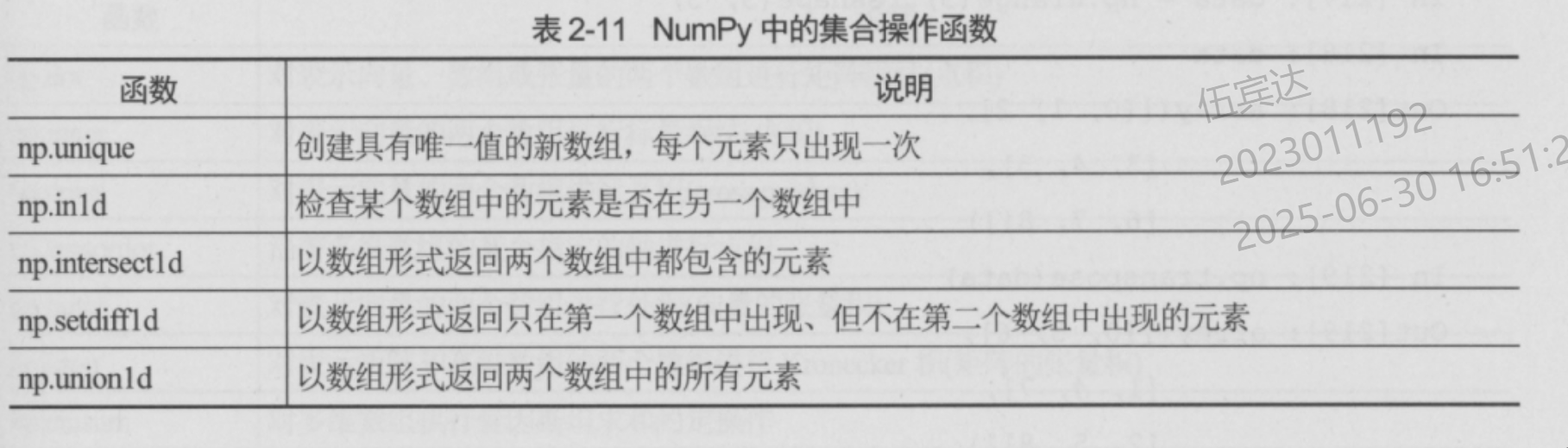
集合运算
数组运算
矩阵和向量运算
| 函数 | 说明 |
|---|---|
| np.dot | |
| np.inner | 向量内积(标量积) |
| np.cross | 向量叉积(注意区分outer) |
| np.tensordot | |
| np.outer | 对表示向量的两个数组进行外积(向量的张量积) |
| np.kron | |
| np.einsum |
矩阵乘法
np.dot或者@符号- 一维数组会视情况解释为shape(1,3)或者shape(3,)
外积
若 (\mathbf{u} \in \mathbb{R}^m),(\mathbf{v} \in \mathbb{R}^n),则外积 (\mathbf{u} \otimes \mathbf{v}) 是一个矩阵 (A_{m \times n}),其中 (A_{ij} = u_i v_j)。
示例:(\mathbf{u} = [1, 2]^\top),(\mathbf{v} = [3, 4, 5]^\top),则:
[
\mathbf{u} \otimes \mathbf{v} = \begin{bmatrix} 3 & 4 & 5 \ 6 & 8 & 10 \end{bmatrix}
]
此运算常用于矩阵分解(如SVD)和协方差计算
Kronecker积
又称克罗内克积或直积,它将两个任意大小的矩阵组合成一个更大的分块矩阵。
1. 基本定义
给定矩阵 ( A \in \mathbb{R}^{m \times n} ) 和 ( B \in \mathbb{R}^{p \times q} ),它们的Kronecker积 ( A \otimes B ) 是一个分块矩阵:
[
A \otimes B = \begin{bmatrix}
a_{11}B & a_{12}B & \cdots & a_{1n}B \
a_{21}B & a_{22}B & \cdots & a_{2n}B \
\vdots & \vdots & \ddots & \vdots \
a_{m1}B & a_{m2}B & \cdots & a_{mn}B
\end{bmatrix}{(mp) \times (nq)}
]
其中每个子块 ( a{ij}B ) 是标量 ( a_{ij} ) 与矩阵 ( B ) 的乘积。结果矩阵的维度为 ( (mp) \times (nq) ) 。
2. 计算示例
设 ( A = \begin{bmatrix} 1 & 2 \ 3 & 4 \end{bmatrix} ),( B = \begin{bmatrix} 0 & 5 \ 6 & 7 \end{bmatrix} ),则:
[
A \otimes B = \begin{bmatrix}
1 \cdot B & 2 \cdot B \
3 \cdot B & 4 \cdot B
\end{bmatrix} = \begin{bmatrix}
0 & 5 & 0 & 10 \
6 & 7 & 12 & 14 \
0 & 15 & 0 & 20 \
18 & 21 & 24 & 28
\end{bmatrix}
]
此例中,( A ) 的每个元素被 ( B ) 的完整副本替换并缩放 。
二、核心性质
Kronecker积满足以下代数性质:
| 性质 | 数学表达 | 意义 |
|------------------|-----------------------------------------------------------------------------|--------------------------------------------------------------------------|
| 分配律 | ( A \otimes (B + C) = A \otimes B + A \otimes C ) | 对矩阵加法的兼容性 |
| 结合律 | ( (A \otimes B) \otimes C = A \otimes (B \otimes C) ) | 支持链式运算 |
| 混合乘积 | ( (A \otimes B)(C \otimes D) = (AC) \otimes (BD) ) | 与矩阵乘法的协同性(需维度匹配) |
| 转置 | ( (A \otimes B)^T = A^T \otimes B^T ) | 转置操作的分配性 |
| 逆矩阵 | ( (A \otimes B)^{-1} = A^{-1} \otimes B^{-1} )(若 ( A, B ) 可逆) | 逆运算的独立性 |
| 特征值 | 若 ( \lambda_i ) 是 ( A ) 的特征值,( \mu_j ) 是 ( B ) 的特征值,则 ( \lambda_i \mu_j ) 是 ( A \otimes B ) 的特征值 | 特征值可分解性 |
| 非交换性 | ( A \otimes B \neq B \otimes A )(一般情况) | 运算顺序影响结果 |
三、应用场景
1. 科学计算与工程领域
- 量子计算:描述多量子比特系统的复合状态(如 ( \psi_{\text{total}} = \psi_1 \otimes \psi_2 ))。
- 信号处理:构造多维滤波器,处理多通道信号(如图像、音频)。
- 图论:生成复杂网络的邻接矩阵(如图的笛卡尔积 ( G_1 \times G_2 ) 的邻接矩阵为 ( A_{G_1} \otimes A_{G_2} ))。
2. 数据分析与机器学习
- 协方差建模:构建高维数据的结构化协方差矩阵(如面板数据 ( \Sigma = \Sigma_{\text{时间}} \otimes \Sigma_{\text{变量}} ))。
- 神经网络加速:通过分块计算简化参数矩阵乘法,提升训练效率(如TensorFlow/PyTorch的
kron函数)。 - 图像处理:实现像素级操作(如2倍放大:用 ( \begin{bmatrix} 1 & 1 \ 1 & 1 \end{bmatrix} ) 与图像矩阵做Kronecker积)。
3. 数值优化
- 大规模线性系统:将高维问题分解为低维子问题(如方程 ( AXB = C ) 转化为 ( (B^T \otimes A) \text{vec}(X) = \text{vec}(C) ))。
- 稀疏矩阵表示:高效存储和计算分块稀疏矩阵 。
1. 基础计算工具
- NumPy:
np.kron(A, B)直接计算,适合中小矩阵 。 - PyTorch/TensorFlow:
torch.kron()或tf.linalg.kronecker,支持GPU加速 。
2. 高性能优化策略
| 场景 | 优化方法 | 目的 |
|---|---|---|
| 大矩阵计算 | 分块算法(Blocking) | 减少内存占用 |
| 并行处理 | 多线程/分布式计算(如Spark) | 加速大规模运算 |
| 稀疏矩阵 | 仅存储非零块 | 节省存储空间 |
| JIT编译 | 使用Numba优化循环 | 提升纯Python代码效率 |
代码示例(NumPy):
import numpy as np
A = np.array([[1, 2], [3, 4]])
B = np.array([[0, 5], [6, 7]])
C = np.kron(A, B)  # 计算Kronecker积
用kronecker积计算外积
- 要获得与np.outer相同的结果,输入的一维数组必须在np.kron的第一、第二个参数扩展为(N,1),(1,N)
爱因斯坦求和约定
二维数组
identity = np.array([[1, 0], [0, 1]])
print(identity)

[out]:[[1 0]
    [0 1]]
二维数组的索引
print(identity[0, 1] is identity[0][1], identity[0, 1] == identity[0][1])

[out]:False True
- 前一种方法是从二维数组中取元素,后一种是先生成一个复制了的一维数组,再取其中的元素,因此 is 判断给出 False ,但它们相等。
square = np.arange(100)
square.shape = (10, 10)
print(square)
- 首先生成了一个长度为 100 的一维数组,随后在保持数据不变的前提下,把它的形状改成了 (10, 10) ,即把它解读成二维方阵。可以理解为数组对象的shape属性是一个tuple,更改了这个属性。
- 这个操作也可以调用 reshape 函数实现:
np.arange(100).reshape((10, 10))
索引取一整行或者列
square[:, 0] # 取出第一列
square[::3, ::5] # 从第一行,列开始每隔3行每隔5列取出元素(Index为3,5倍数的元素,0也匹配)
square[2::3, 3:5] # 从第3(2+1)行开始,每3行取一次
:和::的用法与python的list类似,起始(default值0),终止(default值=维数+1,左闭右开),间隔(default=1)- 当间隔为负数时,例如array[::-1],起始为数组末尾,终止为数组开始。 这很python!!! 符合人类语言。
任意索引(fancy index)
- 分别传两个相等形状的索引数组,按索引数组形状排列对应的输出
print(m6[[1, 2, 3], [3, 4, 5]]) # 给出的新数组的形状由[1,2,3]的形状决定
[out]: [13 24 35]

print(m6[[[1], [2]], [[3], [4]]]) # 输出形状是[[],[]]
[out]:[[13]
       [24]]
数组运算
- 可以对numpy数组做各种操作,+-/……以及+=,-=,=,/=等运算符
降维运算
np.mean()函数用于求数组的均值np.std()函数用于求数组的标准差np.var()求方差np.max()函数用于求数组的最大值np.min()函数用于求数组的最小值np.median()函数用于求数组的中位数np.sum()函数用于求数组的和np.prod()函数用于求数组的积
如果只针对某一个维度,使用axis参数指定
np.sum(square, axis=0), np.mean(square, axis=1)
axis=0表示对每一列求和axis=1表示对每一行求均值- 对于多维数组,
axis参数也可以使用tuple,指定多个维度
矩阵的拓展(广播机制)
n[None, :] + n[:, None]
- 使用
n[None, :]得到:[out]:array([[0, 1, 2, 3, 4, 5, 6, 7, 8, 9]])获得一个二维数组,n[:, None]同理 - 对于两个形状不同的数组,
numpy使用广播机制得到:
array([[ 0, 1, 2, 3, 4, 5, 6, 7, 8, 9],
    [ 1, 2, 3, 4, 5, 6, 7, 8, 9, 10],
    [ 2, 3, 4, 5, 6, 7, 8, 9, 10, 11],
    [ 3, 4, 5, 6, 7, 8, 9, 10, 11, 12],
    [ 4, 5, 6, 7, 8, 9, 10, 11, 12, 13],
    [ 5, 6, 7, 8, 9, 10, 11, 12, 13, 14],
    [ 6, 7, 8, 9, 10, 11, 12, 13, 14, 15],
    [ 7, 8, 9, 10, 11, 12, 13, 14, 15, 16],
    [ 8, 9, 10, 11, 12, 13, 14, 15, 16, 17],
    [ 9, 10, 11, 12, 13, 14, 15, 16, 17, 18]])
矩阵运算
元素乘法与矩阵乘法区别
a = b = np.ones((2,2))
print(a * b) # 对应位置元素相乘,输出[[1 1][1 1]]
print(a @ b) # 矩阵乘法,输出[[2 2][2 2]]
张量
- 矩阵可以表示为两个下标的矩阵元:二阶张量
- 三个下标:三阶张量
eps()
- 反对称张量:
eps(n):返回一个n阶反对称张量对应的高阶矩阵(自定义模块asym.py中)
张量乘法
- np.tensordot(),可标注哪些下标进行缩并(内积操作)
a = np.arange(60).reshape((3,4,5))
b = np.arange(24).reshape((4,3,2))
np.tensordot(a,b,axes = ([0,1],[1,0])) # 合并两个方向,输出为一个二阶张量(6-2*2=2)
爱因斯坦约定
eeinsum:a = np.arange(25).reshape(5,5) b = np.arange(5) np.einsum('ii',a) # 取迹 np.einsum('ij->i', a) # 对j方向求和 np.einsum('ij,i', a,b) # 矩阵乘法# 之前的tensordot等价于如下: np.einsum('ijk,jil',a,b) np.einsum('ijk,jil->kl',a,b)- 灵活缩并
a = np.ones(64).reshape(2,4,8)
np.einsum('ijk,ilm,njm,nlk',a,a,a,a)
#=>4096.0
例:Pauli矩阵
- python中定义的虚数单位
j - numpy中的矩阵乘法运算符
@ - 量子力学中自旋为1/2态空间下的角动量算符表示。
- 这三个矩阵一起,可以看作一个3*2*2的三阶张量
Pauli矩阵的对易关系
pauli = []
pauli.append(np.array([0,1,1,0]).reshape(2,2))
pauli.append(np.array([0,-1j,1j,0]).reshape(2,2))
pauli.append(np.array([1,0,0,-1]).reshape(2,2))
特征值和迹
- NumPy 的 linalg (意为 linear algebra)子模块
np.linalg.eigvals(square) # 计算方阵的特征值
np.trace(square) # 计算方阵的迹
np.linalg.det() # 计算矩阵行列式

- 全反对称张量的含义:
- 全:3*3*3,4*4*4
- 反对称
pauli = np.array(pauli)
(np.einsum('ixy,jxy -> ijxz', pauli,pauli)
- np.einsum('ixy,jxy -> jixz', pauli,pauli)) ==
2j * np.einsum('ijk, kxy', eps(3), pauli) # 或者 np.tensordot(eps(3), pauli, axes = ([2], [0]))
更简单的形式
@符号,重载- 对于矩阵,是矩阵乘法,自动缩并
- 对于张量
# pauli.shape = (3,2,2)
# 对pauli进行拓展:pauli[:,None].shape= (3,1,2,2),pauli[Noen,:].shape = (1,3,2,2)
# 因为之后的两个2*2没有变,所以省略了(pauli[:, None, :, :])
pauli[:, None] - pauli[None, :] # 通过扩展和广播机制,形状变为(3,3,2,2)

# 验证:
np.all(commute(pauli[:, None], pauli[None, :]) ==
        2j * np.tensordot(eps(3), pauli, axes = ([2], [0])))
NumPy 中的 np.stack() 函数用于沿新轴堆叠多个同形状数组,生成一个维度更高的新数组。以下是其核心用法详解:
概述
Pandas库在 NumPy的基础上,补充了很多对数据处理特别有用的功能,如标签索引、分层索引、数据对齐、合并数据集合、处理丢失数据等。因此,Pandas库已经成为Python 中执行高级数据处理的事实标准库,尤其适用于统计应用分析。
一些其他的相关库
statemodels,pasty,scikit-learn:更复杂的统计分析和建模Seabron:强大的统计绘图功能
Pandas中的两大主要数据结构:
Series和DataFrame
导入模块
import numpy as np
import pandas as pd
import matplotlib.pyplot as plt
- 使用一种更美观的绘图样式
import matplotlib as mpl
mpl.style.use('ggplot')
- 导入
seaborn模块
import seaborn as sns
Series对象
基础操作
index,value属性- 与numpy的数组很像
s = pd.Series([98790, 234,57562, 6736])
print(s)
print(s.index)
print(s.values)
- 输出
0    98790
1      234
2    57562
3     6736
dtype: int64
RangeIndex(start=0, stop=4, step=1)
[98790   234 57562  6736]
更具有描述性的方式
- 可以把一个新的索引列表赋值给Series对象的index属性,也可以给 Series 对象的 name 属性设置有意义的名称。
s.index = {"北京", "上海", "广州", "深圳"}
s.name = "评分"
print(s)
print(s.index)
print(s.values)
- 输出
北京    98790
广州      234
上海    57562
深圳     6736
Name: 评分, dtype: int64
Index(['北京', '广州', '上海', '深圳'], dtype='object')
[98790   234 57562  6736]
- 也可以在创建Series的时候就设置索引和名称
s = pd.Series([98790, 234,57562, 6736], name="评分",
            index = ['北京', '广州', '上海', '深圳'])
- 可以通过将索引作为下标来访问数据,也可以直接访问与索引名同名的属性
s['北京']
s.北京
- 使用一个索引列表来访问 Series 对象,将返回一个新的包含原始数据子集(与列表的索引对应)的 Series 对象
s[["北京", "上海"]]
获得Series的统计信息的方法
s.median()
s.mean()
s.std()
s.min()
s.max()
s.quantile()
- 以上所有信息都可以通过
describe()方法统一输出
print(s.describe())
count        4.000000
mean     40830.500000
std      46367.220731
min        234.000000
25%       5110.500000
50%      32149.000000
75%      67869.000000
max      98790.000000
Name: 评分, dtype: float64
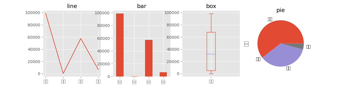
和matplotlib联动进行可视化
- 可以通过 ax 参数把一个 matplotlib Axes 实例传给 plot 方法
- 通过 kind 参数进行设置(可选值有 line、hist、bar、barh、box、kde、density、area 和 pie)
fig, axes = plt.subplots(1,4,figsize=(12,3))
s.plot(ax=axes[0], kind='line', title='line')
s.plot(ax=axes[1], kind='bar', title='bar')
s.plot(ax=axes[2], kind='box', title='box')
s.plot(ax=axes[3], kind='pie', title='pie')

plt.show()
DataFrame对象
DataFrame的初始化
使用嵌套列表
df = pd.DataFrame([[9999,"永州"],[8888,"成都"],[5555,"北京"],[1111,"上[>print(df)
      0   1
0  9999  永州
1  8888  成都
2  5555  北京
3  1111  上海
- 可以通过index设置行索引,通过columns属性来设置列标签
df.columns = ['评分', '城市']
print(df)
     评分  城市
0  9999  永州
1  8888  成都
2  5555  北京
3  1111  上海
使用字典进行初始化
- 列头是字典的键,每列的数据是字典的值
索引
类似于 NumPy 数组使用 values 属性获取数据一样,可以使用 index 和 columns 属性分别获取DataFrame 中数据的索引和所有列,其中的每一列可以使用与列名相同的属性来访。
df["评分"]和df.评分类似
loc索引器
从 DataFrame 中提取一列数据后,将返回一个新的 Series 对象。DataFrame 实例的行可以使用loc索引器属性进行索引。在该属性上进行索引后返回的也是一个 Series 对象,对应原始数据结构中的一行数据:
df.loc[0]
给loc索引器属性传入一个行标签列表后,将返回一个新的 DataFrame,它是原始 DataFrame 的一个子集,里面只包含选择的行。
df.set_index():将索引设置为其他的列
df_pop2 = df_pop.set_index("City")
sort_index():将索引作为关键字对所有数据进行排序
sort_values():根据某列进行排序,关键字ascending设置降序/升序
分层/多层索引
暂时略
统计信息
- 基本统计信息的获取:与Series类似,当调用相关的函数时,DataFrame会对每个数值类型的列进行计算
df.info()方法查看数据集的概要信息- 对于很大的数据集使用
df.head(),df.tail()截取首尾的子集
df.value_counts():对于分类数据进行统计
DataFrame读写数据
CSV文件
read_csv()函数:从.csv文件读取数据并创建DataFrame实例
- 可选参数 参数|作用 ---|--- header| 指定哪一行是列头 skiprows| 跳过开头的几行 delimiter| 每列之间的分隔符 nrows|
待添加
数据转换操作
df.apply()方法
- 把函数传给某列的 apply 方法之后,该函数将作用于该列中的每个元素,生成一个新的 Series 对象并返回。
- 例如,可以传递一个lambda 函数(用于去掉字符串中的“,”字符,并把结果转换为整数类型)给 apply方法,把Population 列的元素从字符串类型转换为整数类型。然后把转换后得到的列赋值给名为NumericPopulation的新列。
- 使用同样的方法,可以对 State 列中的数据进行清洗,再使用 stip 方法去除 State 列中每个元素末尾的空格。
df_pop[“NumericPopulation”] = df_pop.Population.apply(
    lambda x: int(x.replace(',', ''))
)
df_pop["State"] = df_pop["State"].apply(lambda x: x.strip())
时间序列
Seabron图形库
- NumPy 用 loadtxt savetxt ,HDF5 用 File ,JSON 是 load 和 dump 。
csv
- 注意事项:一般的.csv文件的第一行为行头
使用numpy
- numpy中集成了处理csv文件的函数
sq = np.arange(100).reshape((10,10))
数据保存
- savetxt(fname, data, fmt='%.18e', delimiter=' ', newline='\n', header='', footer='', comments='# ', encoding=None)
np.savetxt("s100.txt",sq,fmt="%d") # 使用“%d”增加可读性
np.savetxt("s100_18e.txt",sq) # 默认为"%.18e"18位科学计数法
数据读入
- 使用
np.loadtxt将文本文件直接读取为numpy.ndarray
np.loadtxt("s100.txt", dtype=int) # dtype=int 保证以整数解读文件,否则数字读入时会被暗中转化成浮点型。
# 一些其他类型:int16 int32 int64 float16 float32 float64 float128
print(type(np.loadtxt("s100.txt", dtype=int) )) # =>  <class 'numpy.ndarray'>
使用csv库
import csv
文件读入
path = Path("s100_1.txt")
lines = path.read_text().splitlines() # lines的类型为list
reader = csv.reader(lines) # 迭代器类型
header = next(reader)
- 注意,
csv.reader默认以','作为分隔符 - 自定义分隔符:使用
delimiter=';'参数
path = Path("s100_1.txt")
lines = path.read_text().splitlines()
reader = csv.reader(lines, delimiter=';') # 自定义分隔符
header = next(reader)
HDF5
- HDF5 具有数据的原始(raw)表示,即 HDF 中保存的是与内存同样标准的整数、浮点数,不会有类似 CSV 的精度损失。HDF5 的数据类型自我描述,在读入内存时不需要额外的信息源,因为 HDF5 文件中包含了数据类型和长度等辅助信息。
- 一个h5文件的例子
s100.h5: Hierarchical Data Format (version 5) data HDF5 "s100.h5" { GROUP "/" { DATASET "s100" { DATATYPE H5T_STD_I64LE DATASPACE SIMPLE { ( 10, 10 ) / ( 10, 10 ) } } } } - GROUP可以嵌套,类似于文件夹
- DATASET是多维数组
命令行中查看h5文件
- (bash)
h5dump:Displays HDF5 file contents.-APrint the header and value of attributes; data of datasets is not displayed.
- 在vscode中可以下载相关拓展
- 使用vitables软件
文件写入(基于numpy)
- h5py.File()产生的对象不是字典,但是模拟了字典的接口
- 也有
.keys(),.values()方法
- 也有
- h5文件的dataset,也就是“values”具有类numpy数组属性
基本操作
# 写入一个h5文件
s100 = np.arange(100).reshape((10,10))
with h5py.File("s100.h5","w") as f:
    f["s100"] = s100
- 类似于字典,"GROUP路径"(类似于文件夹目录)作为key,dataset(多维数组)作为value
进阶操作
with h5py.File('data.h5', 'w') as f:  # 'w'模式覆盖写入
    # 创建数据集并写入数组
    dset = f.create_dataset("matrix", data=np.random.rand(100, 100))

    # 添加元数据属性
    dset.attrs["description"] = "100x100 random matrix"

    # 创建组并在组内添加数据集
    grp = f.create_group("experiment")
    grp.create_dataset("temperatures", data=[25.3, 26.1, 24.8])
数据格式转换
- 使用numpy的
.astype(np.int8)转换精度,实现低精度储存,节省内存资源with h5py.File("s100-int8.h5", "w") as opt: opt["s100-int8"] = s100.astype(np.int8)
读取h5
with h5py.File("s100.h5", 'r') as f:
    h5_s100 = f["s100"][...]
print(h5_s100) # =>一个二维数组
print(h5_s100.dtype) # =>int64
[...]或者[()],代表把所有数据读进内存- 把 s100 取出时,HDF5 自我描述可自动把 NumPy 的类型设置好
数据集移动
- 用复制和删除组合实现。我们把 /home/s100 移动到 /s100
with h5py.File("hzg.h5", "a") as ipt:
    ipt["s100"] = ipt["home/s100"]
    del ipt["home/s100"]
访问属性
- 使用读出的数据集的.attrs[]方法
attr_value = dataset.attrs['attribute_name']
 print(attr_value)
 #
遍历所有属性
for key, value in dataset.attrs.items():
 print(f"{key}: {value}")
遍历 HDF5 文件结构
def print_hdf5_structure(name, obj):
    indent = '  ' * name.count('/')
    if isinstance(obj, h5py.Group):
        print(f"{indent}Group: {name}")
    elif isinstance(obj, h5py.Dataset):
        print(f"{indent}Dataset: {name}, shape: {obj.shape}, dtype: {obj.dtype}")

file_path = 'path/to/your/file.h5'
with h5py.File(file_path, 'r') as h5_file:
h5_file.visititems(print_hdf5_structure)
JSON
- 当数据没有整齐形态,可能伴随有分支、嵌套等时,使用JSON更方便
- JSON 借鉴了 Python 字典和列表的语法,与 Python 交互极其方便。
- 但是 JSON 面向的纯文本数据,与 CSV 类似,对数字的表现力弱。
- JSON就是python的字典不断嵌套
JSON读取
open()+json.load()
import json

with open("BBH_events_v3.json", "r") as ipt:
    events = json.load(ipt)
events此时就是一个python字典对象
JSON写入
with open("BBH_events_rewrite.json", 'w') as opt:
    json.dump(events, opt)
Structured Array数组中的符合数据结构
- 见python目录下相关文件
- 复合数组可以直接保存为HDF5的表格,而且可以在vitables或其他数据处理软件中很好地转化为表格
with h5py.File("people.h5", "w") as opt:
    opt['record'] = r
DataFrame表格
- 复合数组是逐行保存地,DataFrame是逐列保存的
- 逐行保存有利于逐步积累数据,HDF5是逐行的
- 逐列保存有利于处理数据,parquet是逐列的
CSV表格
- 读入CSV:
data = np.read_csv("文件名", skiprows=4)- 可选参数
skiprows:跳过指定的行数
- 可选参数
- 可以把复合数组写到CSV中,形成一个表格。
df_r.to_csv("people.csv")
index=False表示不保存行的标号
- 读入使用
pd.read_csv()
Apache Arrow与Parquet
读写parquet
mydataframe.to_parquet("people.pq",index=False)
pq = pd.read_parquet("people.pq")
pandas读写hdf5
- 写入hdf5
ds.to_hdf("osci.h5", ds_name)ds_name为数据集的名字
- 标准的hdf5输出
with h5py.File("osci.h5", "w") as opt:
    # 先转化为复合数组,再写入文件兼容性更好
    opt[ds_name] = ds.to_records(index=False)
    # 写入数据标签
    for k, v in meta.items():
    opt[ds_name].attrs[k] = v
导入模块
import matplotlib as mlp
from matplotlib import pyplot as plt
from mlp_toolkits.mplot3d.axes3d import Axes3D
mlp简介
- matplotlib中的图形由一Figure(画布)实例以及该实例中的多个 Axes(轴)实例构建而成。Figue实例为绘图提供了画布区域,Axes 实例则提供了坐标系,并分配给画布的固定区域
- 一个Figure实例可以包含多个Axes实例
- Axes 实例提供了一个可用于绘制不同样式图形的坐标系,包括线图、散点图、柱状图等样式。另外,Axes 实例还可以用来决定如何显示坐标轴,例如轴标签、刻度线、刻度线标签等。事实上,在使用natplotlib的面向对象 API时,用于设置图形外观的大部分函数都是 Axes 类的方法。
交互与非交互模式
mpl.useuse(backend, *, force=True) Select the backend used for rendering and GUI integration. - interactive backends: GTK3Agg, GTK3Cairo, GTK4Agg, GTK4Cairo, MacOSX, nbAgg, QtAgg, QtCairo, TkAgg, TkCairo, WebAgg, WX, WXAgg, WXCairo, Qt5Agg, Qt5Cairo - non-interactive backends: agg, cairo, pdf, pgf, ps, svg, template- 当使用用于在用户界面中显示图形的交互式后端时,需要调用函数 plt.show() 以在屏幕上显示窗口。默认情况下,plt.show()调用程序将挂起,直到窗口被关闭。
plt.ion():启动交互模式,每次绘图直接显示。plt.ioff():关闭交互模式。- 需要让图形的变动生效,使用
plt.draw()重绘
曲线图
基础操作
plt.plot([1,2,3,4])
plt.show()
- 只画点
plt.plot([1,2,3,4], '.')
- color参数指定颜色
- label参数指定曲线标签
- legend参数显示图例
- 帮助文档
plot([x], y, [fmt], *, data=None, **kwargs)
plot([x], y, [fmt], [x2], y2, [fmt2], ..., **kwargs)

**Markers**
=============   ===============================
``'.'``         point marker
``','``         pixel marker
``'o'``         circle marker
``'v'``         triangle_down marker
``'^'``         triangle_up marker
``'<'``         triangle_left marker
``'>'``         triangle_right marker
``'1'``         tri_down marker
``'2'``         tri_up marker
``'3'``         tri_left marker
``'4'``         tri_right marker
``'8'``         octagon marker
``'s'``         square marker
``'p'``         pentagon marker
``'P'``         plus (filled) marker
``'*'``         star marker
``'h'``         hexagon1 marker
``'H'``         hexagon2 marker
``'+'``         plus marker
``'x'``         x marker
``'X'``         x (filled) marker
``'D'``         diamond marker
``'d'``         thin_diamond marker
``'|'``         vline marker
``'_'``         hline marker
=============   ===============================

**Line Styles**
=============    ===============================
``'-'``          solid line style
``'--'``         dashed line style
``'-.'``         dash-dot line style
``':'``          dotted line style
=============    ===============================
**Colors**
=============    ===============================
``'b'``          blue
``'g'``          green
``'r'``          red
``'c'``          cyan
``'m'``          magenta
``'y'``          yellow
``'k'``          black
``'w'``          white
=============    ===============================
散点图
scatter(x, y, s=None, c=None, marker=None, cmap=None,
        norm=None, vmin=None, vmax=None, alpha=None,
        linewidths=None, *, edgecolors=None,
        plotnonfinite=False, data=None, **kwargs)
s:点的大小(标量或数组,默认值 20)c:点的颜色(字符串、RGB 元组或数值数组)marker:点的形状(如 'o'(圆)、'^'(三角形)、's'(方形))alpha:透明度(0~1)edgecolors:点的边框颜色(如 'k'(黑色))
直方图
hist(x, bins=None, range=None, density=False,
        weights=None, cumulative=False, bottom=None,
        histtype='bar', align='mid', orientation='vertical',
        rwidth=None, log=False, color=None, label=None,
        stacked=False, *, data=None, **kwargs)
bins:整数、序列或字符串(default值10),定义柱子数量或边界- 整数:分箱数
- 序列:自定义每个箱(如 [0, 10, 20],只有两个箱)
- 字符串:自动分箱策略('auto', 'sturges')
density:True 时纵轴显示概率密度(面积和为1)(默认为False)histtype:图形类型,字符串类型'bar':传统柱状(多组并列)'barstacked':多组堆叠'step':未填充线框'stepfilled':填充线框
orientation:方向:'vertical'(垂直)或 'horizontal'(水平)cumulative:累计分布alpha:透明度color / edgecolor
图片注释
图例
- 添加图例
plt.legend()
坐标轴
- 坐标轴范围:
plt.xlim(t.min() * 1.5,t.max() * 1.5) - 坐标轴标签:
plt.xlabel("arc"),plt.ylabel("value")
子图绘制
subplot函数
subplot(nrows, ncols, index, **kwargs)
nrows:子图网格的行数ncols:子图网格的列数index: 当前子图位置索引(从1开始),按行优先从左到右编号**kwargs:其他关键字参数
plt.subplot(2, 2, 1)  # 第1行第1列
plt.plot([1, 2, 3], [4, 5, 6])
plt.subplot(2, 2, 4)  # 第2行第2列
plt.scatter([1, 2, 3], [7, 8, 9])
plt.show()
plt.subplots()更推荐
- 功能:一次性创建网格布局,返回Figure对象和Axes对象数组,支持面向对象操作
subplots(nrows=1, ncols=1, *,
        sharex=False, sharey=False, squeeze=True, width_ratios=None,
        height_ratios=None, subplot_kw=None, gridspec_kw=None, **fig_kw)
    Create a figure and a set of subplots.
sharex/sharey:共享X/Y轴刻度(可设为True、'row'、'col')- 这一点对于子图的美观性还挺重要的
- 不使用共用y轴
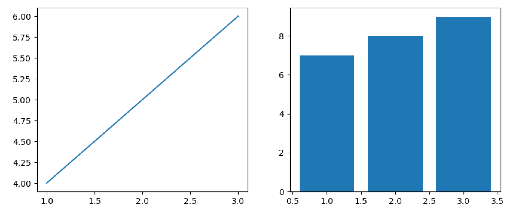
- 使用公用y轴
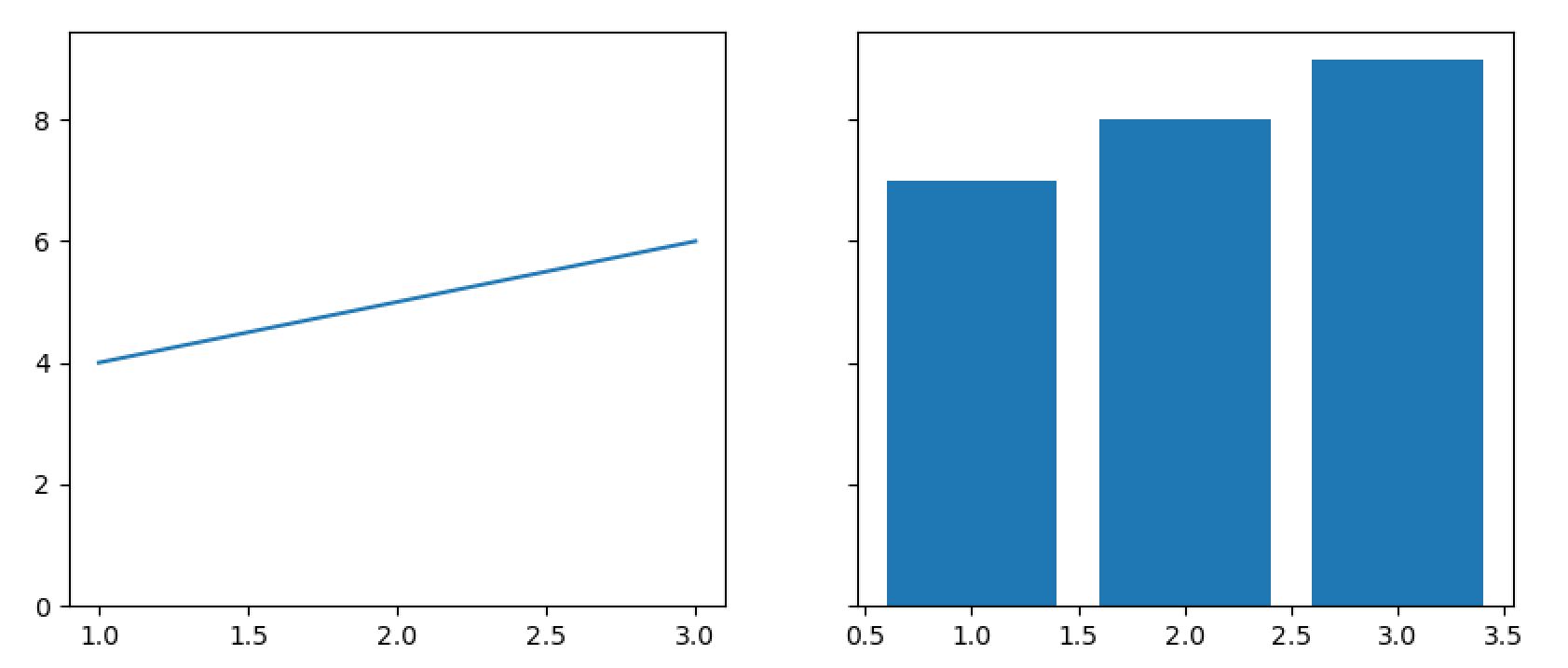
figsize:画布尺寸(宽, 高,单位英寸)
fig, (ax1, ax2) = plt.subplots(1, 2, sharey=True, figsize=(10, 4))
ax1.plot([1, 2, 3], [4, 5, 6])
ax2.bar([1, 2, 3], [7, 8, 9])
表现多维数据
- 通过色块的颜色表现第三维数据的数值大小
- 使用
colorbar函数显示颜色和数值的映射条 - 函数原型:
cbar = plt.colorbar(mappable, ax=ax, cax=cax, **kwargs)- mappable:必选,关联的数据对象(如
im = ax.imshow(data)) ax:指定父坐标系,色条将自动放置在其旁cax:自定义色条坐标系,实现精确布局orientation='horizontal'
- mappable:必选,关联的数据对象(如
imshow()函数
- 将二维数组(如矩阵、图像)渲染为均匀网格色块,适用于规则排布的离散数据或真实图像
plt.imshow(data, cmap='hot', origin='lower', interpolation='nearest')- data的数据格式
- (M, N):灰度图(标量值映射为颜色)。
- (M, N, 3):RGB 彩色图像。
- (M, N, 4):RGBA 图像(含透明度)
- cmap:颜色映射(如 'viridis'、'gray'),将标量值映射为颜色。
- origin:坐标系方向,'upper'(数组左上角为图像左上角,默认)或 'lower'(数组左下角为图像左下角)。
- aspect:纵横比控制,'equal'(像素为方形)或 'auto'(自适应画布)。
- interpolation:像素插值方法(如 'nearest' 保留锐边,'bilinear' 平滑过渡)。
- vmin/vmax:颜色映射的值域范围限制
- data的数据格式
- 注意事项当用 imshow 显示矩阵时,若未设置 origin='lower',图像可能上下翻转(因数组原点在左上角,而笛卡尔坐标系原点在左下角
img = np.arange(100).reshape(10, 10)
plt.imshow(img)
plt.colorbar(img)
- 先通过
plt.imshow(img)指定一个数据对象
例子:多维正态分布,contourf 函数绘制填充等高线图
contourf 函数
- 在二维平面上绘制三维数据的等值线,并在相邻等值线间填充颜色,形成连续色块
绘制多维正态分布
from scipy.stats import multivariate_nor
rv = multivariate_normal(mean=(0, 0),cov = ((1,0.5),(0.5,0.5)))
print(rv.pdf((0, 0))) #(x,y)->f(x,y)
- 创建多元正态分布对象并从指定均值和协方差矩阵
mean=(0, 0):均值向量,表示两个维度的期望值均为0cov=((1, 0.5), (0.5, 0.5)):协方差矩阵,表示:- 第一个维度的方差为 1(对角线元素)。
- 第二个维度的方差为 0.5(对角线元素)。
- 两个维度间的协方差为 0.5(非对角线元素),说明两者存在正相关性
norm_x,norm_y = np.mgrid[-1:1:.01,-1:1:.01]
pos = np.dstack((norm_x,norm_y)) # pos=>(200, 200, 2)三位数组
- 生成二维网格,并沿第三维堆叠
prob_density = rv.pdf(pos)
print(pos.shape,prob_density.shape)
对比
plt.imshow(prob_density)
plt.colorbar()
- 两个函数的原点约定不同,可以使用imshow()的origin参数调整
真三维图
from mpl_toolkits.mplot3d import axes3d
ax = plt.figure().add_subplot(projection='3d')
#Plotthe3D surface
ax.plot_surface(norm_x,norm_y,prob_density,
            edgecolor='royalblue',lw=0.5,
            rstride=8,cstride=8,
            alpha=0.3)
ax.set( xlim=(-1, 1),ylim=(-1, 1),zlim=(0, 0.4),
        xlabel='x',ylabel='y',zlabel='f(x,y)')
plt.show()
流线图
P, Q = np.mgrid[-1:1:.002,-1:1:.002]
dP =-Q # \dot{p}
dQ = P # \dot{q}
plt.streamplot(Q, P, dQ, dP)
多曲线图
- 对一个图不断plot,绘制的曲线会在一张图上叠加
from scipy import special
x = np.linspace(0, 6, 100)
y_values = [special.jv(n,x) for n in range(0, 5)] #第一类Bessel函数
for i,y in enumerate(y_values):
    plt.plot(x,y,label=f"Order {i}")
plt.legend()
plt.xlabel("x")
plt.ylabel("valuesofBesselfunction")
🌪️ 流体力学计算中向量化优化核心方法与注意事项
🔧 向量化替代循环的核心方法
- 网格坐标系统构建
# 正确矩阵索引(避免笛卡尔坐标错误)
i_grid, j_grid = np.meshgrid(
    np.arange(height),
    np.arange(width),
    indexing='ij'  # 关键参数
)
原理:创建(height, width)形状的坐标矩阵,保持与物理场维度一致
- 物理量批量计算
# 向量化回溯位置计算
phys_x = i_grid + 0.5  # 网格中心物理坐标
phys_y = j_grid + 0.5
back_x = phys_x - velocity_x  # 所有点同时计算
back_y = phys_y - velocity_y
- 插值参数向量化
# 批量计算双线性插值参数
x0 = np.floor(back_x).astype(int)
y0 = np.floor(back_y).astype(int)
dx = back_x - x0
dy = back_y - y0
weights = np.stack([(1-dx)*(1-dy), dx*(1-dy), (1-dx)*dy, dx*dy], axis=2)
- 场更新向量操作
# 单指令更新整个场
advected_field = (
    weights[:,:,0] * field[x0, y0] +
    weights[:,:,1] * field[x1, y0] +
    weights[:,:,2] * field[x0, y1] +
    weights[:,:,3] * field[x1, y1]
)
⚠️ 关键注意事项
-
网格索引陷阱
indexing='ij':科学计算标准 (行,列)indexing='xy':笛卡尔标准 (列,行)
错误案例:
# 错误:默认xy导致维度反转 x, y = np.meshgrid(np.arange(width), np.arange(height)) -
边界一致性处理
- 物理坐标转换:网格点位于
(i+0.5, j+0.5) - 安全裁剪:
np.clip(pos, 0, size-1.001)避免索引溢出 - 边界条件:速度场用
factor=-1,压力场用factor=1
- 物理坐标转换:网格点位于
-
内存管理优化
# 避免中间数组副本 result = np.empty_like(input_array) np.multiply(a, b, out=result) # 原地操作 # 大数组分块处理 for i in range(0, height, block_size): block = array[i:i+block_size] # 处理分块 -
数值稳定性保障
- CFL条件:
max(|u|)Δt/Δx < 1 - 浮点精度:使用
np.float64减少累积误差 - 正则化处理:
dyes = np.clip(dyes, 0, 1)
- CFL条件:
NumPy的复合数据类型(Structured Array)是一种强大的数据结构,允许在单个数组中存储异构数据(不同数据类型),类似于数据库表格或结构化记录。以下是其核心特性和使用方法的系统介绍:
🧱 一、核心概念
-
定义与特点
- 异构数据存储:复合数据类型允许每个数组元素包含多个字段(字段名 + 数据类型),例如存储学生信息(姓名:字符串、年龄:整数、成绩:浮点数)。
- 内存高效:基于NumPy的连续内存模型,访问速度快,适合大规模数据处理。
- 字段访问:支持通过字段名直接访问数据(如
array['age']),无需额外转换。
-
适用场景
- 表格数据处理(CSV、数据库导出)
- 科学计算中的多参数记录(如物理实验中时间、位置、温度等)
- 与Pandas DataFrame互操作(结构化数组可无缝转为DataFrame)
🔧 二、创建方法
1. 定义数据类型(dtype)
使用 np.dtype 指定字段结构,支持三种语法:
- 元组列表(最常用):
dtype = np.dtype([('name', 'U10'), ('age', 'i4'), ('height', 'f4')]) - 字典形式:
dtype = np.dtype({'names': ['name', 'age', 'height'], 'formats': ['U10', 'i4', 'f4']}) - 字符串简写:
dtype = np.dtype('U10, i4, f4') # 字段名自动分配为f0, f1, f2
注:U10 表示长度10的Unicode字符串,i4 为32位整数,f4 为32位浮点数。
2. 创建结构化数组
data = np.array([('Alice', 25, 1.65), ('Bob', 30, 1.80)], dtype=dtype)
输出:
[('Alice', 25, 1.65) ('Bob', 30, 1.80)]
3. 三种创建方式对比
| 方法 | 语法示例 | 优势 | 限制 |
|---|---|---|---|
| 元组列表 | dtype=[('name','U10'), ('age','i4')] | 字段名和类型明确 | 代码稍长 |
| 字典形式 | dtype={'names':['name','age'], 'formats':['U10','i4']} | 字段名集中管理 | 不支持嵌套字段 |
| 字符串简写 | dtype='U10, i4, f4' | 简洁 | 字段名默认为f0,f1,... |
🛠️ 三、数据操作
-
字段访问与修改
- 按字段提取列:
names = data['name'] # 输出:['Alice' 'Bob'] - 按行访问:
first_row = data[0] # 输出:('Alice', 25, 1.65) - 修改值:
data['age'] += 1  # 所有年龄+1
data[0]['height'] = 1.70  # 修改Alice身高
- 按字段提取列:
-
切片与条件筛选
# 筛选年龄>25的记录 filtered = data[data['age'] > 25] # 输出:[('Bob', 31, 1.80)] -
排序
# 按年龄升序排序
sorted_data = np.sort(data, order='age')
# 多字段排序:先按年龄,再按身高
sorted_data = np.sort(data, order=['age', 'height'])
⚡ 四、高级特性
-
嵌套字段
支持字段内嵌套复合类型,适合存储树状结构:dtype_nested = np.dtype([ ('info', [('name', 'U10'), ('age', 'i4')]), # 嵌套字段 ('height', 'f4') ]) data_nested = np.array([(('Alice', 25), 1.65)], dtype=dtype_nested) -
多维字段
字段可以是多维数组,用于存储矩阵或张量:dtype_matrix = np.dtype([ ('id', 'i4'), ('matrix', 'f8', (3, 3)) # 每个元素包含3x3矩阵 ]) arr_matrix = np.zeros(2, dtype=dtype_matrix) -
字段增删(需重建数组)
# 添加体重字段
new_dtype = np.dtype(dtype.descr + [('weight', 'f4')])
new_data = np.zeros(data.shape, dtype=new_dtype)
for field in data.dtype.names:
    new_data[field] = data[field]
new_data['weight'] = [55, 70]  # 填充新字段
💡 五、实际应用案例
学生成绩管理系统
# 定义数据类型
dtype = np.dtype([
    ('name', 'U10'),
    ('math', 'f4'),
    ('english', 'f4'),
    ('physics', 'f4')
])

# 创建数组
students = np.array([
    ('Alice', 85, 90, 88),
    ('Bob', 92, 85, 90)
], dtype=dtype)

# 计算平均分并添加新字段
avg_scores = np.mean([students['math'], students['english'], students['physics']], axis=0)
students = np.lib.recfunctions.append_fields(students, 'average', avg_scores, dtypes='f4')
输出:
[('Alice', 85., 90., 88., 87.67) ('Bob', 92., 85., 90., 89.0)]
⚠️ 六、注意事项
- 内存对齐
使用np.dtype(..., align=True)可强制内存对齐(类似C结构体),提升CPU访问效率 - 性能局限
复杂查询(如多条件筛选)效率低于Pandas,建议在数据清洗后转为结构化数组进行计算。 - 类型映射
复合类型可直接映射到C结构体,适合与C/Fortran库交互(如物理仿真、信号处理)。
💎 总结
NumPy复合数据类型通过结构化数组实现异构数据的高效存储,核心价值在于:
- 灵活建模:用单一数组管理多类型数据,避免多数组同步问题。
- 高性能计算:保留NumPy向量化操作优势,支持排序、筛选等复杂操作。
- 跨平台兼容:内存布局兼容C语言,无缝对接底层科学计算库。
import itertools as it
accumulate
it.accumulate(data, function)
data是一个可迭代对象function可以是普通函数,也可以是无名函数lambda- 列子:
max:python自定义的最大值函数;lambda x,y:x+y无名函数
- 列子:
permutations
it.permutations(range(1, 4))
使用zip合并两个迭代器
for i, s in zip(range(11), it.accumulate(range(11))):
    pass
filtertrue和filterfalse:对迭代器进行过滤
it.filterfalse(lambda n: n % 13, range(100))
- SciPy 在 NumPy 的基础上提供的数值计算算法
IPython作为增强型交互式Python环境,提供了大量高效的操作技巧,以下从核心功能维度分类整理,结合实用场景和最佳实践,助你显著提升命令行效率:
🔍 一、智能补全与内省
-
Tab键补全
- 对象属性补全:输入对象名后加
.,按Tab显示所有属性和方法(如"hello".<Tab>展示字符串方法)。 - 模块与路径补全:
- 模块补全:
import numpy as np; np.<Tab>显示NumPy函数列表。 - 文件路径补全:输入路径前缀后按
Tab(如/usr/<Tab>)自动补全目录或文件名。
- 模块补全:
- 动态过滤:输入部分字符(如
ma<Tab>)匹配map、max等函数,减少记忆负担。
- 对象属性补全:输入对象名后加
-
帮助文档与源码查看
- 快速文档:
obj?显示对象文档字符串(如len?查看参数说明)。 - 源码查看:
obj??尝试显示源代码(如str.upper??展示底层实现)。 - 函数签名:输入函数名后加
?直接显示参数列表(如print?)。
- 快速文档:
✨ 二、魔法命令(Magic Commands)
-
代码执行与调试
%run script.py:执行脚本并保留变量到当前会话。%debug:在异常后自动进入调试器,支持n(下一步)、c(继续)、q(退出)。%timeit:多次运行代码计算平均耗时(如%timeit sum(range(1000)))。
-
系统与文件操作
!cmd:执行Shell命令(如!ls或!dir)。%cd /path:切换工作目录,%pwd显示当前路径。%%writefile filename.py:将代码块保存到文件
-
命名空间管理
%who/%whos:列出变量及类型/内存信息。%reset:清空当前会话所有变量。
与系统shell进行交互
- IPython与shell之间的双向通行非常方便
- IPython中不仅可以执行系统shell命令,还可以将执行的结果赋值给python变量
file = ! ls
- 同样,也可以在Python变量名前加<data class="katex-src" value=",从而将python变量传递给shell ```python file = "file1.py" ! ls - ">
IPython扩展
%lsmagic显示所有可用扩展命令
1. 文件系统导航
- 略
2. 在Ipython控制台中运行脚本
%run可以在Ipython中运行外部python脚本,且会将文件中的符号添加到本地命名空间中,由此引入函数模块或类定义。
3. 调试器
%debugger:当未能拦截的异常打印到IPython 控制台后,可使用IPython 的%debug 命令直接进入Python 调试器。- 在 debugger 提示符中输入问号,可以显示帮助菜单,其中列出了可以使用的命令。
4. 代码性能分析
%timeit,%time
⏱ 三、历史操作与快捷键
-
历史命令复用
- 方向键:上下箭头浏览历史命令。
- 反向搜索:
Ctrl+R输入关键词匹配历史命令(如Ctrl+R后输入plot定位绘图代码) %history:显示完整历史记录,支持-n参数过滤行号。
-
编辑快捷键
- 光标控制:
Ctrl+A(行首)、Ctrl+E(行尾)、Ctrl+F/B(前进/后退字符) - 删除操作:
Ctrl+K(删至行尾)、Ctrl+U(删整行)。 - 清屏:
Ctrl+L快速清空终端
- 光标控制:
输入输出缓存
- 输入输出的提示符分别为In[1]和Out[1],[]内的数字会递增。
- 输入输出代码单元可以通过IPython自动生成的In和Out变量来访问。
- In变量是列表,Out变量是字典,元素均为字符串。
🧪 四、高级功能与集成
-
可视化与富文本
%matplotlib inline:内嵌显示Matplotlib图形。display(HTML(...)):渲染HTML/Markdown(如生成表格或公式)
-
性能分析与并行
%load_ext line_profiler+%lprun -f func func():逐行分析函数性能%%parallel:并行执行代码块(需配置IPython集群)
-
模块热重载
%load_ext autoreload+%autoreload 2:修改模块后自动重载,避免重启内核
💎 效率对比与场景推荐
| 功能 | 命令示例 | 适用场景 | 效率提升 |
|---|---|---|---|
| 智能补全 | np.array(<Tab> | 快速探索库功能 | ⭐⭐⭐⭐⭐ |
| 帮助文档 | pd.DataFrame? | 即时查询API用法 | ⭐⭐⭐⭐ |
| 魔法命令计时 | %timeit [...] | 性能优化关键代码 | ⭐⭐⭐⭐ |
| 历史反向搜索 | Ctrl+R + 关键词 | 复用复杂命令 | ⭐⭐⭐ |
| 模块热重载 | %autoreload 2 | 交互式开发调试 | ⭐⭐⭐⭐ |
💡 实践建议:
- 数据分析场景:优先使用
%run加载脚本、%timeit测试性能,结合%matplotlib inline即时可视化。- 调试技巧:异常后立即输入
%debug进入交互调试,用n/c跟踪逻辑。- 扩展性:通过
%load_ext加载ipywidgets等扩展,增强交互能力
常用基础调试
- 直接在python脚本中添加
breakpoint(),运行时会自动暂停并进入pdb调试环境。 - 使用
pdb.set_trace(),可以在代码任意位置设置断点,运行时会自动暂停并进入pdb调试环境。 - 使用
pdb.run('python script.py'),可以直接进入pdb调试环境,并运行指定的python脚本。 - 日志记录:使用
tee保存调试过程到文件:python script.py | tee debug.log
🔧 一、启动调试
1. 侵入式(代码内断点)
在需暂停的代码行插入 pdb.set_trace():
import pdb

def example(a, b):
    result = a + b
    pdb.set_trace()  # 程序运行到此暂停
    return result
直接运行脚本:python script.py[citation:1][citation:2][citation:7]。
2. 非侵入式(命令行启动)
无需修改代码,通过命令启动调试:
python -m pdb script.py
程序会在第一行自动暂停
⌨️ 二、常用调试命令
| 命令 | 简写 | 作用 |
|---|---|---|
next | n | 执行下一行(不进入函数) |
step | s | 执行下一行(进入函数内部) |
continue | c | 继续运行直到下一个断点或结束 |
print | p | 打印变量值(p x) |
list | l | 显示当前代码上下文(默认11行) |
break | b | 设置断点(b 行号或b 函数名) |
where | w | 显示当前调用栈位置 |
return | r | 执行到当前函数返回 |
quit | q | 退出调试器[citation:1][citation:2][citation:5][citation:7] |
⚡ 三、高级调试技巧
-
条件断点
在循环或特定条件下触发断点:for i in range(10): if i > 5: # 当i>5时暂停 pdb.set_trace() print(i)或通过命令设置:
b 10, i>5(在第10行设置条件) -
调用栈操作
w:查看当前调用栈层次。u/d:在调用栈中向上/向下移动(用于多层函数调试)
-
修改变量值
在调试中动态修改变量:(Pdb) !x = 20 # 将x的值改为20 (Pdb) p x 20使用
!避免与命令冲突 -
跳过循环
until或unt 行号:执行到指定行(跳过循环):(Pdb) unt 15 # 执行至第15行
文件str操作常用命令
模式匹配
grep, egrep, fgrep, rgrep- print lines that match patterns
    grep [OPTION...] PATTERNS [FILE...]
    grep [OPTION...] -e PATTERNS ... [FILE...]
    grep [OPTION...] -f PATTERN_FILE ... [FILE...]
tr:translate or delete characters-s:squeeze-repeats
统计操作
-
uniq:report or omit repeated lines-c, --count: prefix lines by the number of occurrences将词频作为前缀
-
wc用于统计输入内容的行数、单词数、字节数等:-l:统计行数(如日志文件行数)。-w:统计单词数(以空格/换行符分隔)。-c:统计字节数(文件大小)。-m:统计字符数(适用于多字节编码如UTF-8)。-L:显示最长行的字符数。
排序
sort:sort lines of text files,按行排序,以\n作为分隔符-d:按字典序排列-n:按字符串的数值排列
控制输出
sed(这个什么都能干)
sudo -i #进入 root 交互环境 退出交互环境的方法:exit 或 logout 或 快捷键 Ctrl + D
标准输出输出与管道、重定向操作
1. 管道符号
- 管道符号:|
- 作用:将前一个命令的输出作为后一个命令的输入
- 限制:默认仅传递正确输出(错误输出stderr需额外处理)
2. wc命令的统计功能
wc 用于统计输入内容的行数、单词数、字节数等:
- 常用选项:
-l:统计行数(如日志文件行数)。-w:统计单词数(以空格/换行符分隔)。-c:统计字节数(文件大小)。-m:统计字符数(适用于多字节编码如UTF-8)。-L:显示最长行的字符数。
- 基础语法:
wc [选项] [文件]  # 直接处理文件
命令 | wc [选项]  # 通过管道处理输入
3. 管道用于筛选
- grep:用于文本搜索和筛选,支持正则表达式。
- 常用选项:
-i:忽略大小写。-v:反向匹配(显示不匹配的行)。-n:显示行号。-r或-R:递归搜索目录。
- 基础语法:
grep [选项] '模式' [文件]
命令 | grep [选项] '模式'
- 常用选项:
4. 用tee保存管道的中间结果
- tee:将标准输出作为标准出入保存到目标文件
seq 100 | grep 7 | tee result.txt | wc -c
5. 重定向
- 重定向标准输出
seq 100 > seq100.txt
cat seq100.txt | head
- 重定向标准输入
wc -l < s100.txt
6. 自由管道 FIFO named pipe
- FIFO(First In, First Out,先进先出),也称为命名管道(Named Pipe),是一种特殊的文件类型,用于进程间通信(IPC, Interprocess Communication)
- 注意文件系统限制
- 切换到支持 FIFO 的本地文件系统(如 /tmp 或用户主目录)
mkfifo filter.pipe
seq 100 > filter.pipe &
grep 7 < filter.pipe
7. 任务控制
jobs查看后台任务&表示运行于后台fg将任务放到前台bg将任务放到后台kill杀死任务Ctrl + C终止前台任务Ctrl + Z暂停前台任务
命令巡礼
1. 本机信息
uname -a查看系统信息hostname查看主机名date查看日期id查看用户信息uptime查看系统运行时间
2. 日常操作
- 创建文件:
touch file1 file2
ls -l file1 file2
3. cut选择列
sudo dmesg | cut -c-15 | tail -n 10
文件信息
find dir -name "*.txt":查找指定目录下的所有 .txt 文件- 识别文件类型
file filename
通配符
*:匹配任意字符(0个或多个)?:匹配单个字符(0个或1个)
脚本
- 让脚本可执行
sed -i '1i #!/bin/bash' script.sh
chmod +x script.sh
第一行为脚本指定 Bash 解释器 '1i' 插入指令:1 表示第一行,i 表示在指定行之前插入内容。 若用 a 则在该行之后插入 Shebang 声明,指定脚本解释器路径。
常见解释器路径
| 解释器路径 | 适用场景 | 示例 |
|---|---|---|
#!/bin/bash | 需 Bash 扩展功能(如数组、正则) | 复杂脚本开发 |
#!/bin/sh | 兼容 POSIX Shell(轻量但功能受限) | 跨平台脚本 |
#!/usr/bin/env python | 调用环境变量中的解释器(增强可移植性) | 多版本 Python 环境 |
chmod +x script.sh 为脚本文件添加可执行权限的命令,使其能够直接运行。
+x:增加执行权限(x表示 execute)。
权限细节
1. 权限类型与范围
- 权限分类:
- 用户(u):文件所有者。
- 组(g):文件所属用户组。
- 其他(o):其他所有用户。
- 所有(a):默认覆盖以上三类(等价于
ugo)。
- 权限类型:
| 符号 | 权限 | 数字值 |
|------|--------|--------|
|r| 读 | 4 |
|w| 写 | 2 |
|x| 执行 | 1 |
2. +x 的实际效果
- 命令行为:
- 为 所有用户(
a)添加执行权限,即chmod a+x script.sh。 - 若需限定范围,可明确指定:
chmod u+x script.sh  # 仅所有者可执行
chmod ug+x script.sh # 所有者及组用户可执行
- 为 所有用户(
脚本的参数
- 脚本调用时的参数,在脚本中使用‘
- 所用参数:
$@
bash变量
a=100
echo $a
b=我是谁
echo <data class="katex-src" value="{a}"><span class="katex"><span class="katex-mathml"><math xmlns="http://www.w3.org/1998/Math/MathML"><semantics><mrow><mi>a</mi></mrow><annotation encoding="application/x-tex">{a}</annotation></semantics></math></span><span class="katex-html" aria-hidden="true"><span class="base"><span class="strut" style="height:0.4306em;"></span><span class="mord"><span class="mord mathnormal">a</span></span></span></span></span></data>{b}
- 变量需要额外的$来指定
- 变量声明时赋值号的左右都不能有空格
变量的引用
- 无引用时,空格起作用
- 单引号时,$没有引用变量作用,只是普通的字符串
- 双引号时,$引用变量的值
a=100
echo "$a" # 输出100
echo '$a' # 输出'<data class="katex-src" value="a'
echo \""><span class="katex"><span class="katex-mathml"><math xmlns="http://www.w3.org/1998/Math/MathML"><semantics><mrow><msup><mi>a</mi><mo mathvariant="normal" lspace="0em" rspace="0em">′</mo></msup><mi>e</mi><mi>c</mi><mi>h</mi><mi>o</mi><mi mathvariant="normal">"</mi></mrow><annotation encoding="application/x-tex">a'
echo "</annotation></semantics></math></span><span class="katex-html" aria-hidden="true"><span class="base"><span class="strut" style="height:0.7519em;"></span><span class="mord"><span class="mord mathnormal">a</span><span class="msupsub"><span class="vlist-t"><span class="vlist-r"><span class="vlist" style="height:0.7519em;"><span style="top:-3.063em;margin-right:0.05em;"><span class="pstrut" style="height:2.7em;"></span><span class="sizing reset-size6 size3 mtight"><span class="mord mtight"><span class="mord mtight">′</span></span></span></span></span></span></span></span></span><span class="mord mathnormal">ec</span><span class="mord mathnormal">h</span><span class="mord mathnormal">o</span><span class="mord">"</span></span></span></span></data>{a}" # 输出100
引用变量的执行结果
$(command):执行命令并将命令运行的标准输出赋值给变量- 分隔的列表被转成由空格分隔
a=<data class="katex-src" value="(seq 100)
echo "><span class="katex"><span class="katex-mathml"><math xmlns="http://www.w3.org/1998/Math/MathML"><semantics><mrow><mo stretchy="false">(</mo><mi>s</mi><mi>e</mi><mi>q</mi><mn>100</mn><mo stretchy="false">)</mo><mi>e</mi><mi>c</mi><mi>h</mi><mi>o</mi></mrow><annotation encoding="application/x-tex">(seq 100)
echo </annotation></semantics></math></span><span class="katex-html" aria-hidden="true"><span class="base"><span class="strut" style="height:1em;vertical-align:-0.25em;"></span><span class="mopen">(</span><span class="mord mathnormal">se</span><span class="mord mathnormal" style="margin-right:0.03588em;">q</span><span class="mord">100</span><span class="mclose">)</span><span class="mord mathnormal">ec</span><span class="mord mathnormal">h</span><span class="mord mathnormal">o</span></span></span></span></data>a
egrep ^23+$表示匹配行首,2固定,3+表示至少有一个3,$表示行尾
n2333=<data class="katex-src" value="(seq 10000 | egrep ^23+"><span class="katex"><span class="katex-mathml"><math xmlns="http://www.w3.org/1998/Math/MathML"><semantics><mrow><mo stretchy="false">(</mo><mi>s</mi><mi>e</mi><mi>q</mi><mn>10000</mn><mi mathvariant="normal">∣</mi><mi>e</mi><mi>g</mi><mi>r</mi><mi>e</mi><msup><mi>p</mi><mn>2</mn></msup><mn>3</mn><mo>+</mo></mrow><annotation encoding="application/x-tex">(seq 10000 | egrep ^23+</annotation></semantics></math></span><span class="katex-html" aria-hidden="true"><span class="base"><span class="strut" style="height:1.0641em;vertical-align:-0.25em;"></span><span class="mopen">(</span><span class="mord mathnormal">se</span><span class="mord mathnormal" style="margin-right:0.03588em;">q</span><span class="mord">10000∣</span><span class="mord mathnormal">e</span><span class="mord mathnormal" style="margin-right:0.03588em;">g</span><span class="mord mathnormal">re</span><span class="mord"><span class="mord mathnormal">p</span><span class="msupsub"><span class="vlist-t"><span class="vlist-r"><span class="vlist" style="height:0.8141em;"><span style="top:-3.063em;margin-right:0.05em;"><span class="pstrut" style="height:2.7em;"></span><span class="sizing reset-size6 size3 mtight"><span class="mord mtight">2</span></span></span></span></span></span></span></span><span class="mord">3</span><span class="mord">+</span></span></span></span></data>)
echo <data class="katex-src" value="n2333
echo "><span class="katex"><span class="katex-mathml"><math xmlns="http://www.w3.org/1998/Math/MathML"><semantics><mrow><mi>n</mi><mn>2333</mn><mi>e</mi><mi>c</mi><mi>h</mi><mi>o</mi></mrow><annotation encoding="application/x-tex">n2333
echo </annotation></semantics></math></span><span class="katex-html" aria-hidden="true"><span class="base"><span class="strut" style="height:0.6944em;"></span><span class="mord mathnormal">n</span><span class="mord">2333</span><span class="mord mathnormal">ec</span><span class="mord mathnormal">h</span><span class="mord mathnormal">o</span></span></span></span></data>{#n2333} # 输出字符个数
bash数组
- 类似于python的列表,可以储存任意元素
busket=()
busket+=( 香蕉 猕猴桃 水蜜桃 西瓜 )
echo ${busket} # 按普通变量取值,只有第一个元素
echo ${busket[3]} # 按数组下标取值
echo ${busket[@]} # 按数组取值,输出所有元素
echo ${#busket[@]} # 输出元素个数
bash字典
- 又称关联数组,类似python的字典
declare -A cargo # 声明字典
cargo[apple]=100
cargo[banana]=200
echo ${cargo[apple]} # 输出 apple 对应的 value
echo ${!cargo[@]} # 输出所有 key
echo ${cargo[@]} # 输出所有 value
bash算术
- 在bash中字符串的使用更便利,万物皆字符串,算数运算需要辅助
- 但比用管道和$()简洁
echo $((1+1)) $((3*5))
echo $(echo 1+3 | bc) $(echo 2*4 | bc)
- 这里bc是外部计算器
- 计算能力有限,只能简单计算
echo $((2**100)) # 输出0
echo $(echo "2^100" | bc) # 输出正确结果
bash程序结构
1. 选择结构
if [ condition1 ]; then
# 条件成立时执行的代码
if [ 3 -gt 2 ]; then
echo "3 大于 2"
else
echo "3 不大于 2"
fi
2. 判断语句
-
[···]是一个程序,与使用test命令等价 -
真假判断来自该程序执行的返回值。
- 返回值:0表示真,非0表示假。与一般的语言正好相反
-
$?or${?}变量值是前一条命令的返回值
test 1 = 2 # false 返回非0
echo $? # 输出非0
test 2 != 3 # true 返回0
echo $? # 输出0
bash内建真假判断
- 内建命令
[[···]],与[···]类似,但支持更多功能 - 内建命令调用速度更快
- 命令层次的逻辑运算
command1 && command2取与command1 || command2取或! command取反
- 逻辑运算可以替代选择结构
[[ 3 -gt 2 ]] && echo "3 大于 2" || echo "3 不大于 2"
&& 逻辑与运算符
- 若左侧命令成功(返回
0),则执行右侧命令;否则跳过。 - 此处因条件为真,执行
echo "3 大于 2"。
|| 逻辑或运算符
- 若左侧命令失败(返回非
0),则执行右侧命令。 - 此处因
&&已成功执行,跳过echo "3 不大于 2"。
3. 循环结构
for循环:
for i in $(seq 10); do
s=$(($s+$y))
x=${y}
y=${s}
done
echo $y
- while循环:
seq 1000 | while read line; do
echo $line | egrep -q '^23+$' && echo $line
done
- until 循环
- 与 while 相似,但条件为假时执行
seq 1000 | until ! read line; do
echo $line | egrep -q '^23+$' && echo $line
done
- 循环控制命令
break:跳出当前循环continue:跳过当前循环,继续下一轮循环
seq 10000 | while read line; do
if echo $line | egrep -q '^23+$'; then
echo "$line,找到匹配."
break
fi
done
bash函数
1. 定义函数
function greet(){
echo "Hello, $1!"
}
2. 函数递归
- 递归计算fabonacci数
- return 给返回值只能用$?捕捉或者用于逻辑运算
function fib(){
if [ $1 -le 2 ]; then
echo 1
else
echo <data class="katex-src" value="(("><span class="katex"><span class="katex-mathml"><math xmlns="http://www.w3.org/1998/Math/MathML"><semantics><mrow><mo stretchy="false">(</mo><mo stretchy="false">(</mo></mrow><annotation encoding="application/x-tex">((</annotation></semantics></math></span><span class="katex-html" aria-hidden="true"><span class="base"><span class="strut" style="height:1em;vertical-align:-0.25em;"></span><span class="mopen">((</span></span></span></span></data>(fib <data class="katex-src" value="(("><span class="katex"><span class="katex-mathml"><math xmlns="http://www.w3.org/1998/Math/MathML"><semantics><mrow><mo stretchy="false">(</mo><mo stretchy="false">(</mo></mrow><annotation encoding="application/x-tex">((</annotation></semantics></math></span><span class="katex-html" aria-hidden="true"><span class="base"><span class="strut" style="height:1em;vertical-align:-0.25em;"></span><span class="mopen">((</span></span></span></span></data>1-1))) + <data class="katex-src" value="(fib "><span class="katex"><span class="katex-mathml"><math xmlns="http://www.w3.org/1998/Math/MathML"><semantics><mrow><mo stretchy="false">(</mo><mi>f</mi><mi>i</mi><mi>b</mi></mrow><annotation encoding="application/x-tex">(fib </annotation></semantics></math></span><span class="katex-html" aria-hidden="true"><span class="base"><span class="strut" style="height:1em;vertical-align:-0.25em;"></span><span class="mopen">(</span><span class="mord mathnormal" style="margin-right:0.10764em;">f</span><span class="mord mathnormal">ib</span></span></span></span></data>(($1-2)))))
fi
}
echo $(fib 10)
3. bash的代码块与子进程
- {```}代表一个代码块,可以把多行代码合成为一个总单元
- (```)使用复刻(fork)一个bash运行代码。
- 子bash中的变量设置不影响外层bash
s=1
(s=2;)
echo $s # 输出1
- 类似于
$(seq 100)代表复刻后运行seq提取标准输出
bash调试
- 除了直接交互和使用echo输出中间结果之外:
set -xv开启调试模式,set +xv关闭调试模式,bash -xv script.sh以调试模式执行脚本。- -vprint 设立了input lines as they are read.
- -xprint commands and their arguments as they are executed.
Make要素
- 基本语法单元
target: sources
program source target # 必须tab键起始,记录数据处理的流程
- target和sources都应对应于当前路径下的文件名
- 当source存在时可以通过program source target来生成target
变量
1. 变量取值
a:=1 # eager evaluation(= 是lazy evaluation)
$(info $(a))
- 调用时使用(info TEXT) 输出TEXT
- 特殊变量:
$^表示输出数据,$@表示输出数据
target: source
program $^ $@
target: source1 source2 source3
program $< --reference $(word 2,$^) --location $(word 3,$^) -o $@
2. make的函数
- 函数调用
$(function arg1 arg2 ···)- word函数:返回第n个参数
$(word N,TEXT)
$(word 2,make.c use.c high.c) # 输出make.c- patsubst函数:替换符合条件的字符串
$(patsubst pattern,replacement,text)
$(patsubst %.c,%.o,make.c use.c high.c) # 输出make.o use.o high.o- foreach函数:遍历参数
$(foreach var,list,text)
$(foreach var,a b c,$(var) $(var)) # 输出a a b b c c- if函数:条件判断
$(if condition,true_part,false_part)
$(if $(findstring a,abc),yes,no) # 输出yes- call函数:调用其他Makefile文件
$(call function,arg1,arg2,···)
$(call my_function,arg1,arg2) - word函数:返回第n个参数
通配符与替换
1. 一般匹配关系pattern
%:匹配任何字符串,包括空字符串*:匹配零个或多个字符?:匹配零个或一个字符
例子
filelist:=x.h5 y.h5 z.h5
.PTHNY: all
all: $(filelist:.h5=.png)
%.png: %.h5
./plot_celestial.py $^ -0 $@
$(filelist:.h5=.png):替换.h5为.png- 也可以用
$(patsubst %.h5,%.png,$(filelist))来实现 - 有共同前缀时可以进一步简写:
$(filelist:.h5=.png)
- 也可以用
- all是一个总括目标
特殊目标
.PHONY:代表无对应文件的目标,用于声明 all 是一个伪目标(Phony Target)- all 通常是 Makefile 的第一个目标,直接运行 make 时会自动执行它。声明为伪目标可确保其可靠性。
DELETE_ON_ERROR:如果出错就把坏文件删掉.SECONDARY保留中间结果
新工具:guile
- 动态生成依赖关系:传统 Makefile 需手动维护依赖,而 Scheme 可自动扫描源码头文件生成依赖树:
%.o: %.c
$(guile (generate-deps $<)) # 调用 Scheme 函数动态生成依赖
gcc -c $< -o $@
- 独立脚本开发
#!/usr/bin/guile -s
!#
(define (factorial n)
(if (<= n 1) 1 (* n (factorial (- n 1)))))
(display (factorial 5)) ; 输出 120
函数式编程:把目标描述清楚
- Makefile 是函数式编程Functional Programming的语言
# 生成 numbers-N.csx 包含N*100+1 到 (N+1)*100 的数字
numbers-%.csv:
seq $(guile (+ 1 (* $* 100))) $(guile (* 100 (+ $* 1))) > $@
total-%: numbers-%.csv
paste -s -d + < $^ | bc > $@
# 求积
prod: total-0 total-1 total-2
paste -s -d* < $^ | bc > $@
Make机理
1. 调试
- 使用
remake - 机理见讲义
简化语句
- Makefile 中可以调用shell命令将其标准输出作为值
sequence:=$(shell seq -w 00 99)
filelist:=$(shell find . -name "*.h5")
- 构造total-N目标
seqs:=$(shell seq 0 2)
totals:=$(seqs:%=total-%)
#另一种方法
totals:=$(addprefix total-,$(seqs))
替换语法
| 语法 | 示例 | 作用 | 适用场景 |
|---|---|---|---|
$(var:%=prefix-%) | $(seqs:%=total-%) | 为每个元素添加固定前缀 | 批量生成新目标名 |
$(var:suffix=) | $(files:.o=.c) | 替换后缀(需精确匹配) | 源文件与目标文件转换 |
$(patsubst pat,rep,$(var)) | $(patsubst %,total-%,$(seqs)) | 通用模式替换(功能同示例) | 复杂模式匹配 |
Makefile脚本
1. 选择结构
a:=$(if CONDITION,THEN-PART[,ELSE-PART])
$(or CONDITON1 CONDITION2),and COND1 COND2用于逻辑运算
2. 循环结构与自定义函数
- 数据本身可以构造一重循环,当循环多于一重时,使用
profile:=<data class="katex-src" value="(foreach d,x y z,"><span class="katex"><span class="katex-mathml"><math xmlns="http://www.w3.org/1998/Math/MathML"><semantics><mrow><mo stretchy="false">(</mo><mi>f</mi><mi>o</mi><mi>r</mi><mi>e</mi><mi>a</mi><mi>c</mi><mi>h</mi><mi>d</mi><mo separator="true">,</mo><mi>x</mi><mi>y</mi><mi>z</mi><mo separator="true">,</mo></mrow><annotation encoding="application/x-tex">(foreach d,x y z,</annotation></semantics></math></span><span class="katex-html" aria-hidden="true"><span class="base"><span class="strut" style="height:1em;vertical-align:-0.25em;"></span><span class="mopen">(</span><span class="mord mathnormal" style="margin-right:0.10764em;">f</span><span class="mord mathnormal">ore</span><span class="mord mathnormal">a</span><span class="mord mathnormal">c</span><span class="mord mathnormal">h</span><span class="mord mathnormal">d</span><span class="mpunct">,</span><span class="mspace" style="margin-right:0.1667em;"></span><span class="mord mathnormal">x</span><span class="mord mathnormal" style="margin-right:0.04398em;">yz</span><span class="mpunct">,</span></span></span></span></data>(rl:%=1t_+%_<data class="katex-src" value="(d).h5))
"><span class="katex"><span class="katex-mathml"><math xmlns="http://www.w3.org/1998/Math/MathML"><semantics><mrow><mo stretchy="false">(</mo><mi>d</mi><mo stretchy="false">)</mo><mi mathvariant="normal">.</mi><mi>h</mi><mn>5</mn><mo stretchy="false">)</mo><mo stretchy="false">)</mo></mrow><annotation encoding="application/x-tex">(d).h5))
</annotation></semantics></math></span><span class="katex-html" aria-hidden="true"><span class="base"><span class="strut" style="height:1em;vertical-align:-0.25em;"></span><span class="mopen">(</span><span class="mord mathnormal">d</span><span class="mclose">)</span><span class="mord">.</span><span class="mord mathnormal">h</span><span class="mord">5</span><span class="mclose">))</span></span></span></span></data>(info <data class="katex-src" value="(profile))
```
- Makefile模板,起到函数作用
```makefile
define video
"><span class="katex"><span class="katex-mathml"><math xmlns="http://www.w3.org/1998/Math/MathML"><semantics><mrow><mo stretchy="false">(</mo><mi>p</mi><mi>r</mi><mi>o</mi><mi>f</mi><mi>i</mi><mi>l</mi><mi>e</mi><mo stretchy="false">)</mo><mo stretchy="false">)</mo><mi mathvariant="normal">‘</mi><mi mathvariant="normal">‘</mi><mi mathvariant="normal">‘</mi><mo>−</mo><mi>M</mi><mi>a</mi><mi>k</mi><mi>e</mi><mi>f</mi><mi>i</mi><mi>l</mi><mi>e</mi><mtext>模板,起到函数作用</mtext><mi mathvariant="normal">‘</mi><mi mathvariant="normal">‘</mi><mi mathvariant="normal">‘</mi><mi>m</mi><mi>a</mi><mi>k</mi><mi>e</mi><mi>f</mi><mi>i</mi><mi>l</mi><mi>e</mi><mi>d</mi><mi>e</mi><mi>f</mi><mi>i</mi><mi>n</mi><mi>e</mi><mi>v</mi><mi>i</mi><mi>d</mi><mi>e</mi><mi>o</mi></mrow><annotation encoding="application/x-tex">(profile))
```
- Makefile模板,起到函数作用
```makefile
define video
</annotation></semantics></math></span><span class="katex-html" aria-hidden="true"><span class="base"><span class="strut" style="height:1em;vertical-align:-0.25em;"></span><span class="mopen">(</span><span class="mord mathnormal">p</span><span class="mord mathnormal">ro</span><span class="mord mathnormal" style="margin-right:0.10764em;">f</span><span class="mord mathnormal">i</span><span class="mord mathnormal" style="margin-right:0.01968em;">l</span><span class="mord mathnormal">e</span><span class="mclose">))</span><span class="mord">‘‘‘</span><span class="mspace" style="margin-right:0.2222em;"></span><span class="mbin">−</span><span class="mspace" style="margin-right:0.2222em;"></span></span><span class="base"><span class="strut" style="height:0.8889em;vertical-align:-0.1944em;"></span><span class="mord mathnormal" style="margin-right:0.10903em;">M</span><span class="mord mathnormal" style="margin-right:0.03148em;">ak</span><span class="mord mathnormal">e</span><span class="mord mathnormal" style="margin-right:0.10764em;">f</span><span class="mord mathnormal">i</span><span class="mord mathnormal" style="margin-right:0.01968em;">l</span><span class="mord mathnormal">e</span><span class="mord cjk_fallback">模板,起到函数作用</span><span class="mord">‘‘‘</span><span class="mord mathnormal" style="margin-right:0.03148em;">mak</span><span class="mord mathnormal">e</span><span class="mord mathnormal" style="margin-right:0.10764em;">f</span><span class="mord mathnormal">i</span><span class="mord mathnormal" style="margin-right:0.01968em;">l</span><span class="mord mathnormal">e</span><span class="mord mathnormal">d</span><span class="mord mathnormal">e</span><span class="mord mathnormal" style="margin-right:0.10764em;">f</span><span class="mord mathnormal">in</span><span class="mord mathnormal">e</span><span class="mord mathnormal" style="margin-right:0.03588em;">v</span><span class="mord mathnormal">i</span><span class="mord mathnormal">d</span><span class="mord mathnormal">eo</span></span></span></span></data>(1)/%.avi: <data class="katex-src" value="(1)/%.mp4
ffmpeg -i "><span class="katex"><span class="katex-mathml"><math xmlns="http://www.w3.org/1998/Math/MathML"><semantics><mrow><mo stretchy="false">(</mo><mn>1</mn><mo stretchy="false">)</mo><mi mathvariant="normal">/</mi><mi>f</mi><mi>f</mi><mi>m</mi><mi>p</mi><mi>e</mi><mi>g</mi><mo>−</mo><mi>i</mi></mrow><annotation encoding="application/x-tex">(1)/%.mp4
ffmpeg -i </annotation></semantics></math></span><span class="katex-html" aria-hidden="true"><span class="base"><span class="strut" style="height:1em;vertical-align:-0.25em;"></span><span class="mopen">(</span><span class="mord">1</span><span class="mclose">)</span><span class="mord">/</span><span class="mord mathnormal" style="margin-right:0.10764em;">ff</span><span class="mord mathnormal">m</span><span class="mord mathnormal">p</span><span class="mord mathnormal">e</span><span class="mord mathnormal" style="margin-right:0.03588em;">g</span><span class="mspace" style="margin-right:0.2222em;"></span><span class="mbin">−</span><span class="mspace" style="margin-right:0.2222em;"></span></span><span class="base"><span class="strut" style="height:0.6595em;"></span><span class="mord mathnormal">i</span></span></span></span></data>$^ $<data class="katex-src" value="@
endef
"><span class="katex"><span class="katex-mathml"><math xmlns="http://www.w3.org/1998/Math/MathML"><semantics><mrow><mi mathvariant="normal">@</mi><mi>e</mi><mi>n</mi><mi>d</mi><mi>e</mi><mi>f</mi></mrow><annotation encoding="application/x-tex">@
endef
</annotation></semantics></math></span><span class="katex-html" aria-hidden="true"><span class="base"><span class="strut" style="height:0.8889em;vertical-align:-0.1944em;"></span><span class="mord">@</span><span class="mord mathnormal">e</span><span class="mord mathnormal">n</span><span class="mord mathnormal">d</span><span class="mord mathnormal">e</span><span class="mord mathnormal" style="margin-right:0.10764em;">f</span></span></span></span></data>(eval <data class="katex-src" value="(foreach d,up down transverse,"><span class="katex"><span class="katex-mathml"><math xmlns="http://www.w3.org/1998/Math/MathML"><semantics><mrow><mo stretchy="false">(</mo><mi>f</mi><mi>o</mi><mi>r</mi><mi>e</mi><mi>a</mi><mi>c</mi><mi>h</mi><mi>d</mi><mo separator="true">,</mo><mi>u</mi><mi>p</mi><mi>d</mi><mi>o</mi><mi>w</mi><mi>n</mi><mi>t</mi><mi>r</mi><mi>a</mi><mi>n</mi><mi>s</mi><mi>v</mi><mi>e</mi><mi>r</mi><mi>s</mi><mi>e</mi><mo separator="true">,</mo></mrow><annotation encoding="application/x-tex">(foreach d,up down transverse,</annotation></semantics></math></span><span class="katex-html" aria-hidden="true"><span class="base"><span class="strut" style="height:1em;vertical-align:-0.25em;"></span><span class="mopen">(</span><span class="mord mathnormal" style="margin-right:0.10764em;">f</span><span class="mord mathnormal">ore</span><span class="mord mathnormal">a</span><span class="mord mathnormal">c</span><span class="mord mathnormal">h</span><span class="mord mathnormal">d</span><span class="mpunct">,</span><span class="mspace" style="margin-right:0.1667em;"></span><span class="mord mathnormal">u</span><span class="mord mathnormal">p</span><span class="mord mathnormal">d</span><span class="mord mathnormal">o</span><span class="mord mathnormal" style="margin-right:0.02691em;">w</span><span class="mord mathnormal">n</span><span class="mord mathnormal">t</span><span class="mord mathnormal" style="margin-right:0.02778em;">r</span><span class="mord mathnormal">an</span><span class="mord mathnormal">s</span><span class="mord mathnormal" style="margin-right:0.03588em;">v</span><span class="mord mathnormal">erse</span><span class="mpunct">,</span></span></span></span></data>(call video,$(d))))
以下是关于 awk 和 paste 命令的详细解释,结合它们在 Linux/Unix 系统中的核心功能、语法和典型应用场景:
1. awk:文本处理编程语言
awk 是一种强大的文本扫描和处理工具,支持变量、函数、条件判断等编程特性,适用于数据抽取、格式化和报告生成。
核心特性
- 逐行处理:
读取输入(文件、管道或标准输入)的每一行,分割为字段(默认以空格分隔),通过$1、$2等引用字段,$0表示整行。 - 脚本结构:
awk 'BEGIN {预处理} /模式/ {动作} END {后处理}' 文件BEGIN:处理前执行(如初始化变量)模式 {动作}:匹配模式时执行操作(如$1 > 100)END:所有行处理完成后执行(如汇总结果)。
- 内置变量:
NR(当前行号)、NF(当前行字段数)、FS(输入字段分隔符)、OFS(输出字段分隔符)。 - 多分隔符支持:
通过-F指定复杂分隔符(如awk -F'[,-]'使用逗号或连字符分割)。
典型应用
- 数据提取:
awk '{print $1, $3}' data.txt(输出第1、3列) - 条件过滤:
awk '$3 > 100 {print $0}' sales.txt(筛选第3列大于100的行) - 数学运算:
awk '{sum += $1} END {print sum}' numbers.txt(计算总和) - 自定义函数:支持定义函数处理复杂逻辑(如计算平均值)。
2. paste:多文件行合并工具
paste 用于将多个文件的对应行横向合并(默认以制表符分隔),适合快速拼接文本数据。
核心特性
- 并行合并:
paste file1.txt file2.txt # 输出:file1的行1 + Tab + file2的行1 - 串行合并(
-s选项):
将单个文件的所有行合并为一行:paste -s file.txt # 输出:行1 Tab 行2 Tab 行3... - 自定义分隔符(
-d选项):paste -d':@' file1 file2 # 用 `:` 分隔第一组,`@` 分隔第二组 - 支持标准输入:
ls | paste -d, - - - # 将`ls`输出按每行3列显示,逗号分隔
典型应用
- 合并日志:
paste timestamps.log errors.log > combined.log - 表格化输出:
ls /etc | paste - - - - -(5列显示目录内容) - CSV生成:
paste -d',' names ages > users.csv
3. awk vs paste 对比总结
| 特性 | awk | paste |
|---|---|---|
| 定位 | 编程语言,支持复杂文本处理 | 命令行工具,专注多文件行合并 |
| 核心功能 | 字段分割、条件过滤、数学运算、报告生成 | 横向拼接行,简单格式化 |
| 分隔符控制 | 支持多分隔符(-F)和正则表达式 | 支持单字符分隔符(-d) |
| 典型场景 | 数据清洗、统计、自定义报表 | 日志合并、多列显示、快速数据拼接 |
| 复杂度 | 高(需学习语法) | 低(即学即用) |
4. 联合使用示例
-
统计日志错误次数并格式化:
grep "ERROR" app.log | awk '{print $1}' | sort | uniq -c | paste -d' ' - -grep过滤含 “ERROR” 的行awk提取时间戳(假设第1列)sort | uniq -c统计次数paste将两列合并为一行输出。
-
生成CSV报告:
awk '{print $1}' names.txt | paste -d, - ages.txt > report.csv
常见问题
awk处理大文件:因逐行处理,内存占用低,适合大型日志。paste的换行问题:Windows 文件(\r\n)可能导致输出错位,需转换为 Unix 格式(dos2unix)。
通过结合 awk 的字段处理能力和 paste 的行合并功能,可高效解决多数文本处理需求。进一步学习可参考 GNU 官方文档或实践案例。
grep(Global Regular Expression Print)文本搜索工具,用于在文件或输入流中快速定位匹配指定模式(字符串或正则表达式)的行。
🔍 一、核心功能与语法
1. 核心能力
- 文本搜索:快速匹配包含关键词的行。
- 正则表达式支持:支持基本(BRE)和扩展正则(ERE,通过
-E),实现复杂模式匹配(如 IP 地址、邮箱格式)。 - 递归搜索:
-r或-R选项可遍历目录及其子目录下所有文件。
⚙️ 二、常用选项详解
以下为高频选项分类说明:
1. 匹配控制
| 选项 | 作用 | 示例 |
|---|---|---|
-i | 忽略大小写 | grep -i "error" log.txt |
-v | 反向匹配(排除行) | grep -v "debug" log.txt |
-w | 全词匹配 | grep -w "test" file.txt(不匹配"testing") |
-o | 仅输出匹配部分 | grep -o "http://[^ ]*" url.txt(提取URL) |
2. 输出格式化
| 选项 | 作用 | 示例 |
|---|---|---|
-n | 显示行号 | grep -n "TODO" code.py |
-l | 仅显示文件名 | grep -rl "deprecated" /src |
-c | 统计匹配行数 | grep -c "404" access.log |
--color | 高亮匹配文本(默认启用) | grep "warning" syslog |
3. 上下文控制
| 选项 | 作用 | 示例 |
|---|---|---|
-A N | 显示匹配行后N行 | grep -A 3 "crash" app.log |
-B N | 显示匹配行前N行 | grep -B 2 "timeout" app.log |
-C N | 显示匹配行前后各N行 | grep -C 2 "exception" app.log |
4. 正则表达式模式
- 基本正则(BRE):默认支持
^(行首)、$(行尾)、.(任意字符)、*(0次或多次)。grep "^2023" log.txt # 匹配以"2023"开头的行 - 扩展正则(ERE):
-E支持+(1次或多次)、?(0或1次)、|(或逻辑)。grep -E "error|warn" log.txt # 匹配含"error"或"warn"的行
🛠️ 三、典型应用场景
1. 日志分析
- 提取错误信息:
grep "ERROR" app.log。 - 统计异常频率:
grep -c "Timeout" api.log。 - 查看错误上下文:
grep -C 5 "segfault" system.log(显示前后5行)。
2. 代码审查
- 递归搜索函数调用:
grep -rn "calculate_score()" /src。 - 列出待修复文件:
grep -l "deprecated" *.js。
3. 数据清洗
- 提取结构化数据:
grep -Eo "[0-9]{1,3}\.[0-9]{1,3}\.[0-9]{1,3}\.[0-9]{1,3}" access.log | sort | uniq -c` # 提取IP并统计出现次数 - 过滤无效数据:
grep -v "N/A" dataset.csv > cleaned.csv。
4. 系统监控
- 实时日志过滤:
tail -f /var/log/syslog | grep --color "Failed login"
⚡️ 四、进阶技巧
1. 组合命令
- 与
find联用:搜索特定扩展名文件内容find /var/log -name "*.log" -exec grep "oom_killer" {} + - 多条件管道过滤:
dmesg | grep "error" | grep -v "USB" # 排除USB相关错误
2. 性能优化
- 限制匹配数:
grep -m 100 "pattern" largefile.log(仅输出前100个匹配)。 - 跳过二进制文件:
grep -I -r "text" /dir(避免解析二进制文件)。
3. 复杂正则
- 匹配邮箱:
grep -Eo "\b[A-Za-z0-9._%+-]+@[A-Za-z0-9.-]+\.[A-Z]{2,}\b" contacts.txt
⚙️ 一、Sed简介
Sed(Stream Editor) 是Linux/Unix系统中的流式文本编辑器,以非交互方式逐行处理文本,执行查找、替换、删除、插入等操作。其核心特点是高效处理大文件,通过模式空间(Pattern Space)缓存当前处理行,编辑后输出结果,不直接修改源文件(除非使用 -i 选项)
🛠️ 二、核心功能与语法
1.常用选项
| 选项 | 作用 |
|---|---|
-n | 抑制默认输出,仅打印处理过的行(常与 p 命令联用) |
-e | 执行多条命令(例:sed -e 's/a/b/' -e 's/c/d/') |
-i[.bak] | 直接修改源文件(.bak 为备份后缀) |
-r | 启用扩展正则表达式(支持 +、? 等元字符) |
-f | 从文件读取脚本命令 |
2. 地址范围控制
通过行号或正则表达式限定操作范围:
- 单行:
sed '5s/old/new/'(仅第5行替换) - 行区间:
sed '1,10d'(删除1-10行) - 模式匹配:
sed '/error/d'(删除含"error"的行) - 混合定位:
sed '/start/,/end/s/old/new/'(匹配start到end的行替换)
⚡️ 三、常用操作命令
1. 替换文本(s 命令)
sed 's/原文本/新文本/[标志]' 文件
- 标志:
g:全局替换(默认仅替换每行首个匹配)p:打印替换后的行(需配合-n)- 数字:替换第N个匹配(例:
s/apple/orange/2替换每行第二个"apple")
# 将所有"apple"替换为"orange"并保存原文件备份
sed -i.bak 's/apple/orange/g' fruits.txt
2. 删除行(d 命令)
# 删除空行
sed '/^$/d' file.txt
# 删除注释行(以#开头)
sed '/^#/d' config.ini
# 删除第3行
sed '3d' log.txt
3. 插入与追加文本
- 插入(
i\):在指定行前添加 - 追加(
a\):在指定行后添加
# 在第2行前插入
sed '2i\插入内容' file.txt
# 在含"section"的行后追加
sed '/section/a\追加内容' config.ini
4. 打印文本(p 命令)
# 打印第5-10行
sed -n '5,10p' log.txt
# 打印含"ERROR"的行
sed -n '/ERROR/p' app.log
5. 行号处理(= 命令)
# 打印含"warning"的行号
sed -n '/warning/=' messages.log
🔧 四、高级技巧
1. 多命令执行
# 方式1:分号分隔
sed 's/a/b/; s/c/d/' file.txt
# 方式2:-e 选项
sed -e 's/a/b/' -e 's/c/d/' file.txt
2. 引用变量
# 双引号支持变量扩展
new="orange"; sed "s/apple/$new/g" file.txt
# 单引号需拼接变量
sed 's/apple/'"$new"'/g' file.txt
3. 正则表达式分组
使用 \(...\) 捕获内容,\1 引用分组:
# 提取IP地址(匹配inet后的内容)
ifconfig ens33 | sed -n 's/.*inet \(.*\) net.*/\1/p'
4. 多行处理
通过 N(读取下一行)、D(删除模式空间首行)等命令合并多行:
# 将空行分隔的记录合并为单行
sed '/./!{H;$!d}; x; s/\n/ /g' data.txt
🧩 五、实战案例
-
批量修改配置文件
# 替换所有.conf文件中的旧IP sed -i 's/192.168.1.1/192.168.1.2/g' /etc/*.conf ``` -
清理日志文件
# 删除3天前的日志(日期格式YYYY-MM-DD) three_days_ago=$(date -d "3 days ago" +%Y-%m-%d) sed -i "/^$three_days_ago/d" app.log -
提取HTML链接
sed -n 's/.*href="\([^"]*\)".*/\1/p' index.html -
备份并修改文件
# 修改前创建.bak备份 sed -i.bak 's/TMOUT=300/TMOUT=0/' /etc/profile
⚠️ 六、注意事项
- 备份文件:使用
-i.bak避免误操作丢失数据。 - 特殊字符转义:替换内容含
/时改用#或@作分隔符(例:s#/old#/new#g)。 - 性能优化:大文件处理时避免复杂正则,优先使用
awk或perl - 测试验证:正式执行前移除
-i测试输出,确认无误后再修改源文件。
Sed的精髓在于**“以行为单位的流式处理”**,结合正则表达式可高效解决90%的文本编辑需求。复杂场景(如JSON解析)建议结合
jq或Python工具
python3 -m venv base # 创建名为myenv的虚拟环境
source base/bin/activate # 激活后命令行显示(myenv)
deactivate # 退出虚拟环境
🔧 一、基础调试方法:追踪命令执行
-
-x选项(Xtrace 模式)- 作用:逐行打印执行前的命令(变量已展开),显示实际执行的指令。
- 启用方式:
或在脚本内局部启用:bash -x script.sh # 命令行启用#!/bin/bash set -x # 开启调试 echo "调试区域" set +x # 关闭调试 - 输出示例:
+ echo 'Hello World' Hello World
-
-v选项(Verbose 模式)- 作用:打印原始命令(未展开变量),与
-x结合使用更全面:bash -vx script.sh # 同时显示原始命令和执行结果
- 作用:打印原始命令(未展开变量),与
⚡ 二、增强调试技巧
-
自定义调试信息格式(
PS4变量)- 默认输出为
+,可改为包含文件名、行号、函数名等:
输出示例:export PS4='+ [${BASH_SOURCE}:${LINENO} in ${FUNCNAME[0]}]: ' set -x+ [script.sh:10 in main]: echo "调试中"
- 默认输出为
-
重定向调试日志到文件
避免终端输出混乱,将追踪信息写入文件:exec 5> debug.log # 创建文件描述符5指向日志文件 BASH_XTRACEFD="5" # 指定调试输出到描述符5 set -x -
局部调试(子Shell隔离)
仅调试脚本片段,避免全局干扰:( set -x; command1; command2 ) # 子Shell内启用调试
🛡️ 三、严格模式(预防性调试)
组合选项提升脚本健壮性,提前暴露问题:
set -euxo pipefail
-e:命令失败时立即退出脚本。-u:使用未定义变量时报错(防止空变量)。-o pipefail:管道中任意命令失败则整个管道失败。
适用于生产环境脚本,避免隐藏错误。
🐞 四、高级调试工具
- 静态检查工具
shellcheck
提前检测语法和潜在问题:shellcheck script.sh # 输出警告和建议
💎 调试模式最佳实践
- 渐进定位:先用
-x定位大致范围,再结合PS4精细化调试。 - 错误捕获:使用
trap '错误处理命令' ERR拦截错误并输出上下文。 - 日志分级:区分调试日志(
>&2输出到标准错误)和正常输出。 - 生产环境:调试后务必关闭调试模式(
set +x),避免泄露敏感信息。
示例:调试一个数据处理函数
#!/bin/bash set -euo pipefail PS4='+ [${LINENO}]: ' # 显示行号 process_data() { set -x [ ! -f "$1" ] && echo "文件不存在" >&2 # ... 处理逻辑 set +x } trap 'echo "错误发生在行 $LINENO" >&2' ERR process_data "input.txt"
掌握这些技巧,可快速解决大部分 Bash 脚本问题。简单调试用 -x 和 set,复杂场景用 bashdb,预防错误用严格模式组合。
命令行输入技巧
Ctrl + U: 从光标处删除到行首Ctrl + K: 从光标处删除到行尾
emacs --batch l1.org -f org-html -export-to-html
sudo apt install lynx # Debian/Ubuntu
lynx your_file.html # 打开文件
在Linux系统中,PATH环境变量定义了Shell在查找可执行文件时的搜索路径。若脚本或程序位于PATH指定的目录中,用户可直接通过命令名调用它,无需输入完整路径。以下结合用户示例命令 file $(which egrep) 详细解析其原理和工作流程:
🔍 一、PATH环境变量的核心作用
-
目录列表与搜索顺序
PATH是由冒号分隔的目录路径列表(如/usr/bin:/bin:/usr/local/bin)。当输入命令(如egrep)时,Shell按顺序遍历这些目录:- 先在
/usr/bin中搜索egrep - 若未找到,继续搜索
/bin,依此类推。 - 找到第一个匹配的可执行文件后立即执行,并停止搜索。
- 先在
-
为何需要
PATH
避免每次执行命令都输入完整路径(如/bin/egrep),提升操作效率。例如:echo $PATH # 查看当前PATH配置
⚙️ 二、命令解析:file $(which egrep)
此命令分为两步执行:
-
which egrep:定位egrep的绝对路径which命令在PATH目录中搜索egrep,返回其完整路径(如/bin/egrep)。- 若
egrep在PATH中不存在,which无输出,导致后续file命令报错。
-
file /bin/egrep:分析文件类型file命令检查路径对应的文件类型(如可执行文件、脚本、二进制等)。- 例如输出:
/bin/egrep: ELF 64-bit LSB executable(二进制可执行文件)或POSIX shell script(脚本)。
🔄 三、Shell查找命令的完整流程
当输入egrep时,Shell的查找顺序为:
- 检查是否为Shell内置命令(如
cd,echo) - 查找哈希表(缓存已执行命令的路径,加速搜索)。
- 遍历
PATH目录:- 依次检查每个目录是否存在
egrep文件。 - 若找到且具有可执行权限(
x),则执行。
- 依次检查每个目录是否存在
- 未找到的异常处理:
- 若所有目录均未找到,返回
command not found。
- 若所有目录均未找到,返回
⚠️ 四、关键注意事项
-
可执行权限
文件必须在PATH中 且 拥有可执行权限(通过chmod +x添加)。ls -l /bin/egrep # 查看权限(应含`x`标志) -
路径优先级
PATH中靠前的目录优先级更高。例如:- 若
/usr/local/bin/egrep和/bin/egrep同时存在,优先执行/usr/local/bin/egrep。
- 若
-
安全性风险
- 避免将当前目录
.加入PATH,否则恶意脚本可能被意外执行。 - 谨慎添加非信任目录,防止路径劫持攻击。
- 避免将当前目录
💡 五、扩展应用场景
- 查找命令的真实位置:
which python # 返回Python解释器路径(如/usr/bin/python) which -a node # 显示所有同名命令的路径(多版本共存时) - 验证脚本类型:
file $(which myscript.sh) # 检查脚本是二进制还是Shell/Python脚本 - 调试路径问题:
若命令未找到,检查:echo $PATH # 确认目录是否包含 ls -l /path/to/command # 检查文件是否存在及权限
🌐 六、which的替代工具
| 命令 | 功能 | 示例 |
|---|---|---|
whereis | 查找二进制、源码及手册路径 | whereis grep(显示/bin/grep及手册位置) |
type | 区分命令类型(内置/别名/外部) | type ls(显示ls is aliased to...) |
command -v | 兼容性更好的命令定位工具 | command -v egrep |
💎 总结
PATH机制是Linux命令执行的基石:
- ✅
which egrep:依赖PATH定位命令路径。 - ✅
file $(...):通过路径分析文件属性。 - ✅ 脚本可执行+在
PATH中:是直接通过命令名调用的前提。 - ⚠️ 安全提示:定期审查
PATH配置,避免包含高危目录。
通过
file $(which command)可快速验证命令的物理位置及文件类型,是排查执行问题的实用技巧。
Bash 脚本的参数是向脚本传递输入的核心机制,通过特殊变量和解析工具实现灵活控制。以下从参数类型、访问方式、解析技术到最佳实践进行系统介绍:
⚙️ 一、参数类型与访问方式
-
位置参数
- 定义:按顺序传递的参数,通过
$1、$2...$n访问。 - 示例:
./script.sh arg1 arg2 # $1="arg1", $2="arg2" - 特殊变量:
$0:脚本自身名称(如./script.sh)$#:参数总数(如2)$@:所有参数的独立列表(推荐用"$@"保留空格分隔的参数完整性)$*:所有参数合并为单个字符串(用空格连接)
$@与$*的区别:
| 场景 |"$@"|"$*"|
|----------------|----------------------------|----------------------------|
| 参数带空格 | 保留独立性(如"arg 1") | 合并为"arg 1 arg2"|
| 循环遍历 | 每个参数单独处理 | 整体作为单个字符串处理 | - 定义:按顺序传递的参数,通过
-
选项参数
- 短选项:以单连字符开头(如
-v、-f file.txt) - 长选项:以双连字符开头(如
--verbose、--file=file.txt) - 标志参数:布尔型选项(如
-h显示帮助)
- 短选项:以单连字符开头(如
🔍 二、参数解析技术
1. 直接访问位置参数
适用场景:参数数量固定且顺序明确。
echo "第一个参数: $1"
echo "第二个参数: $2"
2. 循环遍历参数
for循环 +$@(推荐处理带空格的参数):for arg in "$@"; do echo "参数: $arg" doneshift命令:左移参数,逐项处理(适合不定数量参数):while [ "$#" -gt 0 ]; do echo "当前参数: $1" shift # 丢弃$1,$2变为$1 done
3. 解析选项参数:getopts
功能:标准化解析带值的选项(如 -a value)。
while getopts ":a:b:" opt; do
case $opt in
a) echo "选项a的值: $OPTARG" ;; # $OPTARG 获取选项值
b) echo "选项b的值: $OPTARG" ;;
?) echo "无效选项: -$OPTARG" ;;
esac
done
说明:
:表示选项需参数(如-a value)- 解析后使用
shift $((OPTIND-1))跳过已处理选项
4. 复杂选项解析:getopt
适用场景:支持长选项(如 --file)和可选参数:
TEMP=$(getopt -o a:b:c --long file:,help -n "脚本名" -- "$@")
eval set -- "$TEMP" # 重组参数
while true; do
case "$1" in
--file) file="$2"; shift 2 ;;
--help) show_help; exit 0 ;;
--) shift; break ;;
esac
done
🛠️ 三、实用技巧与最佳实践
-
参数验证
- 检查数量:避免缺少参数导致错误:
if [ $# -lt 2 ]; then echo "需提供至少2个参数!" exit 1 fi - 空参数处理:
-z "$1"检测空参数
- 检查数量:避免缺少参数导致错误:
-
默认值与帮助信息
name="默认名" # 设置默认值 usage() { echo "用法: $0 [-n 名称]"; exit 1; } while getopts ":n:" opt; do case $opt in n) name="$OPTARG" ;; ?) usage ;; esac done -
封装脚本的参数传递
封装脚本需转发所有参数(如egrep封装grep -E):#!/bin/sh exec grep -E "$@" -
安全提示
- 验证用户输入的参数(如检查文件是否存在
[ -f "$1" ]) - 避免直接执行未过滤的参数(防命令注入)
- 验证用户输入的参数(如检查文件是否存在
💻 四、综合示例
#!/bin/bash
# 解析选项和位置参数
while getopts ":v" opt; do
case $opt in v) verbose=1 ;; esac
done
shift $((OPTIND-1))
# 验证位置参数
if [ $# -eq 0 ]; then
echo "错误:需提供文件名!" >&2
exit 1
fi
# 处理文件
for file in "$@"; do
[ "$verbose" ] && echo "处理文件: $file"
wc -l "$file"
done
执行:
./count_lines.sh -v file1.txt "file 2.txt"
✅ 总结
- 基础访问:位置参数(
$1,$#,$@)是核心; - 进阶解析:
getopts处理短选项,getopt支持长选项; - 健壮性:验证参数、设置默认值、生成帮助信息;
- 场景适配:简单脚本用位置参数,复杂逻辑用选项解析。
在编程语言设计中,eager evaluation(及早求值) 和 lazy evaluation(惰性求值) 是两种核心的表达式计算策略。你给出的例子 a := 1 属于 eager evaluation,而 = 在特定上下文(如函数式语言或延迟赋值场景)可能隐含 lazy evaluation。以下是详细解释:
⚙️ 1. Eager Evaluation(及早求值)
- 核心机制:表达式在绑定到变量时立即计算,结果直接存储。
例如:
a := 1 + 2 * 3
计算步骤:- 先计算
2 * 3 = 6; - 再计算
1 + 6 = 7; - 最终
a被赋值为7。
- 先计算
- 特点:
- 即时性:赋值时即完成所有计算。
- 内存高效:结果存储后,原始表达式内存可释放。
- 典型语言:C、Java、Python 等传统语言默认采用此策略。
⛓️ 2. Lazy Evaluation(惰性求值)
- 核心机制:表达式延迟计算,直到其结果被实际使用时才执行。
例如:
b = 1 + 2 * 3(在支持惰性的语言中)b绑定的是表达式1 + 2 * 3本身,而非结果7;- 当后续代码调用
b时(如print(b)),才触发计算。
- 特点:
- 按需计算:避免不必要的计算(如未使用的表达式)。
- 支持无限数据结构:例如生成无限序列的迭代器。
- 典型应用:
- Haskell、Scheme 等函数式语言;
- JavaScript 迭代器(如
generator); - 数据库字段按需加载(Lazy Fetching)。
🧩 3. 为什么 a := 1 是 Eager,而 = 可能是 Lazy?
a := 1:1是常量,无需计算,但赋值操作本身是立即生效的(变量a直接存储1),符合 eager 特性。
=的惰性场景:- 在支持惰性的语言中,
=可能仅绑定表达式而非结果。例如:; Scheme 示例:define 绑定表达式,计算延迟到调用时 (define x (+ 1 2)) ; x 绑定为表达式 (+ 1 2),未立即计算 (print x) ; 此时才计算并输出 3 - 代理模式(Proxy):某些语言通过代理对象隐藏延迟计算细节(如 C++ 中的惰性向量运算)。
- 在支持惰性的语言中,
⚖️ 4. 两种策略的优缺点对比
| 特性 | Eager Evaluation | Lazy Evaluation |
|---|---|---|
| 计算时机 | 立即执行 | 按需执行 |
| 内存占用 | 结果存储后释放表达式内存 ✅ | 需保存未计算的表达式结构 ❌ |
| 性能 | 避免重复计算(结果可复用) ✅ | 避免无效计算(如未使用的表达式) ✅ |
| 适用场景 | 确定性计算、实时系统 | 大型数据集、无限序列、条件加载 |
| 调试复杂度 | 执行顺序直观 ✅ | 执行流分散(难追踪计算触发点) ❌ |
🛠️ 5. 实际应用场景示例
- 避免重复复制(Lazy Copy):
// C++ 字符串惰性复制:仅在修改时创建副本 String s1 = "Hello"; String s2 = s1; // 共享数据,未立即复制 s2[0] = 'h'; // 修改时触发复制 - 无限序列生成(Lazy Iterator):
// JavaScript 生成无限偶数序列 function* evenNumbers() { let n = 0; while (true) yield n += 2; } const nums = evenNumbers(); console.log(nums.next().value); // 2(仅计算一次) - 条件加载(Lazy Fetching):
// 数据库对象按需加载字段 class LargeObject { mutable string* field1Value; // 延迟加载指针 const string& field1() const { if (!field1Value) loadField1(); // 使用时才加载 return *field1Value; } };
💎 总结
a := 1是典型的 eager evaluation:赋值即完成计算,结果立即可用。=在惰性语境中:可能绑定未计算的表达式(如函数式语言),实际计算推迟到值被使用时触发。- 选择策略:
- 追求实时性 → Eager(如系统编程);
- 优化资源消耗 → Lazy(如大数据处理、函数式编程)。
理解两种策略的差异,有助于在开发中根据场景选择高效的计算模型,避免不必要的性能损耗。
在虚拟机中设置中文输入法,需根据虚拟机操作系统(Windows/Linux)和虚拟化软件(VMware/VirtualBox)进行配置。以下是具体步骤及常见问题解决方案:
⚙️ 一、Windows 虚拟机设置中文输入法
-
安装中文语言包
- 打开 设置 → 时间和语言 → 语言 → 添加语言,选择“中文(简体)”并安装语言包。
- 将中文设为默认语言,重启生效。
-
添加中文输入法
- 在 语言 设置中点击中文的 选项 → 添加键盘,选择“微软拼音”或“搜狗输入法”。
- 通过
Win+空格切换输入法。
-
调整区域设置
- 控制面板 → 区域 → 格式 选项卡选择“中文(简体,中国)”。
- 管理 选项卡 → 更改系统区域设置,选择“中文(简体)”。
-
安装字体(可选)
- 若中文字体显示异常,在 控制面板 → 字体 中安装“Microsoft YaHei”等字体。
🐧 二、Linux 虚拟机设置中文输入法(以 Ubuntu/CentOS 为例)
第一步:安装中文语言支持
- Ubuntu:
sudo apt update sudo apt install language-pack-zh-hans # 安装简体中文包 sudo dpkg-reconfigure locales # 勾选 zh_CN.UTF-8 - CentOS:
重启系统生效。sudo yum install langpacks-zh_CN # 安装中文包 sudo localectl set-locale LANG=zh_CN.UTF-8
第二步:选择输入法框架(Fcitx 或 IBus)
- Fcitx(推荐,支持搜狗输入法):
sudo apt purge ibus # 卸载冲突的 IBus sudo apt install fcitx fcitx-config-gtk fcitx-pinyin # 安装 Fcitx 及拼音 - IBus(轻量级):
安装后重启。sudo apt install ibus ibus-pinyin # Ubuntu sudo yum install ibus ibus-pinyin # CentOS
第三步:安装具体输入法
- 系统拼音:
sudo apt install fcitx-pinyin # Fcitx 拼音 sudo apt install ibus-pinyin # IBus 拼音 - 搜狗输入法(仅 Fcitx):
重启系统。sudo apt install libqt5qml5 libqt5quick5 # 安装依赖 wget http://cdn2.ime.sogou.com/dl/sogoupinyin_4.x.x_amd64.deb sudo dpkg -i sogoupinyin*.deb # 安装 DEB 包 sudo apt --fix-broken install # 修复依赖
第四步:配置输入法
- Fcitx:
- 右上角系统托盘点击键盘图标 → Configure → 移除默认输入法,添加 Sogou Pinyin 或 Pinyin。
- 设置切换快捷键(如
Ctrl+空格)。
- IBus:
- 终端输入
ibus-setup→ 输入法 选项卡添加 Chinese (Pinyin)。 - 设置快捷键(如
Super+空格)。
- 终端输入
🔧 三、虚拟机软件优化设置
| 虚拟化软件 | 关键操作 |
|---|---|
| VMware | 安装 VMware Tools:菜单选择 虚拟机 → 安装 VMware Tools,挂载镜像后执行安装命令。 |
| VirtualBox | 安装 增强功能:菜单选择 设备 → 安装增强功能,提升输入兼容性。 |
| 通用设置 | 启用 3D 加速(VMware/VirtualBox 虚拟机设置 → 显示 → 启用 3D 加速),避免输入法候选框不显示。 |
⚠️ 四、常见问题与解决
| 问题现象 | 解决方案 |
|---|---|
| 输入法无法切换 | 检查快捷键冲突(如 Ctrl+空格 被占用),在输入法设置中修改快捷键。 |
| 候选框不显示 | 禁用虚拟机 3D 加速(部分系统兼容性差)。 |
| 部分应用无法输入中文 | 启动命令前加环境变量:env GTK_IM_MODULE=fcitx QT_IM_MODULE=fcitx XMODIFIERS=@im=fcitx 应用名。 |
| 中文乱码 | 确保系统语言编码为 zh_CN.UTF-8,安装中文字体包(如 fonts-wqy-microhei)。 |
| 输入法框架冲突 | 卸载冗余框架(如同时安装 Fcitx 和 IBus 时,保留其一)。 |
💎 五、操作总结
graph LR
A[选择系统] --> B{Windows or Linux?}
B -->|Windows| C[安装语言包→添加输入法→设区域]
B -->|Linux| D[装语言包→选框架→安输入法→配置]
D --> E[Fcitx + 搜狗]
D --> F[IBus + 拼音]
C & E & F --> G[虚拟机优化: 3D加速/VMware Tools]
G --> H[测试输入法]
提示:
- 优先使用 Fcitx + 搜狗输入法(Linux 下体验最佳)。
- 操作涉及系统配置时,建议提前创建 虚拟机快照 以防配置错误。
- 若仍遇问题,检查系统日志:
tail -f /var/log/syslog # Ubuntu journalctl -xe # CentOS
-
zsh-autosuggestions(搭配 Oh My Zsh)- 功能:基于输入历史实时提示完整命令,按
→键补全。 - 安装:
# 先安装 Oh My Zsh sh -c "$(curl -fsSL https://raw.github.com/ohmyzsh/ohmyzsh/master/tools/install.sh)" # 启用插件 git clone https://github.com/zsh-users/zsh-autosuggestions ${ZSH_CUSTOM:-~/.oh-my-zsh/custom}/plugins/zsh-autosuggestions - 配置:在
~/.zshrc中添加plugins=(... zsh-autosuggestions)。
- 功能:基于输入历史实时提示完整命令,按
-
fish-shell- 功能:内置自动补全引擎,无需配置即可智能提示命令、参数和路径。
- 安装:
# Debian/Ubuntu sudo apt install fish # 设为默认 Shell chsh -s $(which fish)
🔍 一、查看进程
1. ps 命令(静态查看)
- 功能:显示当前进程快照,支持多种筛选和格式化输出。
- 常用选项组合:
ps aux:显示所有用户进程的详细信息(BSD 风格),包括 CPU/内存占用、启动命令等。ps -ef:以完整格式显示进程树(System V 风格),包含父进程 PID(PPID)。ps -eo pid,user,%cpu,%mem --sort=-%mem:按内存占用降序排序,自定义输出列。
- 示例:
ps aux | grep nginx # 过滤包含 "nginx" 的进程 ps -p 1234 -o comm= # 显示 PID 1234 的进程名(无列名)
2. top / htop(动态监控)
- 功能:实时刷新进程状态和资源占用(CPU、内存等)。
- 交互命令:
P:按 CPU 使用率排序,M:按内存使用率排序。k:终止指定 PID 的进程(默认发送SIGTERM)。r:调整进程优先级(输入nice值)。
- 高级用法:
top -d 5 -o %MEM # 每 5 秒刷新,按内存排序 htop -u mysql # 仅显示 mysql 用户的进程(需安装 `htop`)
3. pgrep(快速定位 PID)
- 功能:根据进程名、用户等属性查找 PID。
- 常用选项:
pgrep -l firefox:显示进程名和 PID。pgrep -u root -x sshd:精确匹配 root 用户的sshd进程。
- 示例:
pgrep -f "java -jar app.jar" # 匹配完整命令行
4. pstree(进程树)
- 功能:以树状结构展示父子进程关系,便于排查依赖或僵尸进程。
- 常用选项:
pstree -p:显示 PID。pstree -s 1234:从 PID 1234 向上追溯父进程链。
- 示例:
pstree -p | grep defunct # 查找僵尸进程
⚔️ 二、终止进程
1. kill(按 PID 终止)
- 信号类型:
kill 1234:默认发送SIGTERM(15),允许进程清理后退出。kill -9 1234:发送SIGKILL(9),强制立即终止(无清理机会)
- 步骤:
# 先查 PID,再终止 pid=$(pgrep -x nginx) kill -15 $pid
2. pkill / killall(按名称终止)
- 功能:批量终止同名进程。
- 示例:
pkill -9 firefox # 强制终止所有 firefox 进程] killall -u testuser # 终止 testuser 的所有进程(`killall` 需安装)]
⚙️ 三、进程控制进阶
1. 后台运行与管理
- 启动后台进程:
sleep 60 & # 末尾加 `&` 后台运行,输出作业编号如 [1] 1234 - 管理后台作业:
jobs # 查看后台作业列表 fg %1 # 将作业 1 调回前台 bg %1 # 让暂停的作业 1 在后台继续运行
2. 调整优先级
nice:启动时设置优先级(-20最高,19最低)。nice -n 10 ./script.sh # 以低优先级运行renice:修改运行中进程的优先级。renice -n 5 -p 1234 # 将 PID 1234 的优先级设为 5